Is Modern Warming Unprecedented? A Critical Look at Holocene Temperature Evidence
Claims that today’s Arctic or global temperatures are unprecedented in the Holocene are still widely repeated in scientific literature. In this article, Andy May examines temperature proxy records and shows that both the magnitude and the rate of warming during the Holocene have been misrepresented.
I find it amazing that some papers still state:
“air temperatures in the [Arctic or globally] are now at their warmest in the past 6,800–7,800 y, and that the recent rate of temperature change is unprecedented over the entire Holocene.” (Lecavalier et al., 2017)
While it is remotely possible that current Arctic or global average temperature is higher than any seen in the past 6,800 years, it is very unlikely and can’t be demonstrated with data we have today. It is almost certainly true that the rate of change in global or Arctic temperature observed recently is not unprecedented in the Holocene Epoch. This modern myth has been thoroughly debunked in the literature and seeing it pop up in PNAS and elsewhere is disconcerting. I thought peer-review was supposed to catch such errors.
Warmest in the past 6,800-7,800 years
The first assertion in Lecavalier et al.’s paper is that the Arctic is now warmer than at any time in the past 6,800-7,800 years. The warmest time in the Holocene (12,000 years ago to the present) is generally accepted to be the Holocene Climatic Optimum or the Holocene Thermal Maximum, both names are used. Two of my favorite Northern Hemisphere Holocene temperature proxies suggest that today is only warmer than the past 1,000-2,000 years as shown in figure 1.
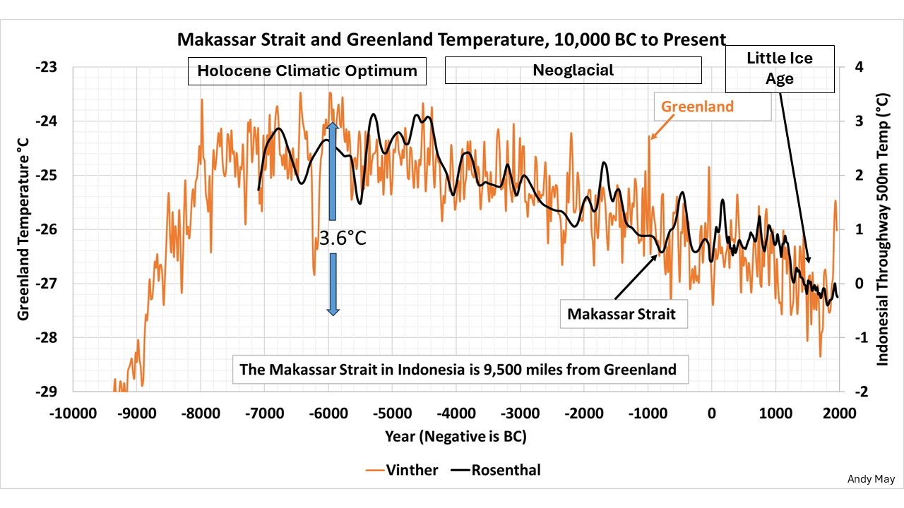
Figure 1. The Vinther Greenland ice core (orange) and the Rosenthal Makassar Strait (black) temperature proxies. Sources: (Vinther et al., 2009) & (Rosenthal et al., 2013).
In figure 1 the Rosenthal Makassar Strait proxy represents sea surface temperature (SST) in the Northern Pacific and the Vinther Greenland proxy is an air temperature proxy in northern Greenland (more details on Vinther and Rosenthal can be seen here). Kaufman et al. (2009) show us a set of Arctic proxies and show them combined in figure 2, which is from the corrected version of the Kaufman, 2009 supplementary materials.
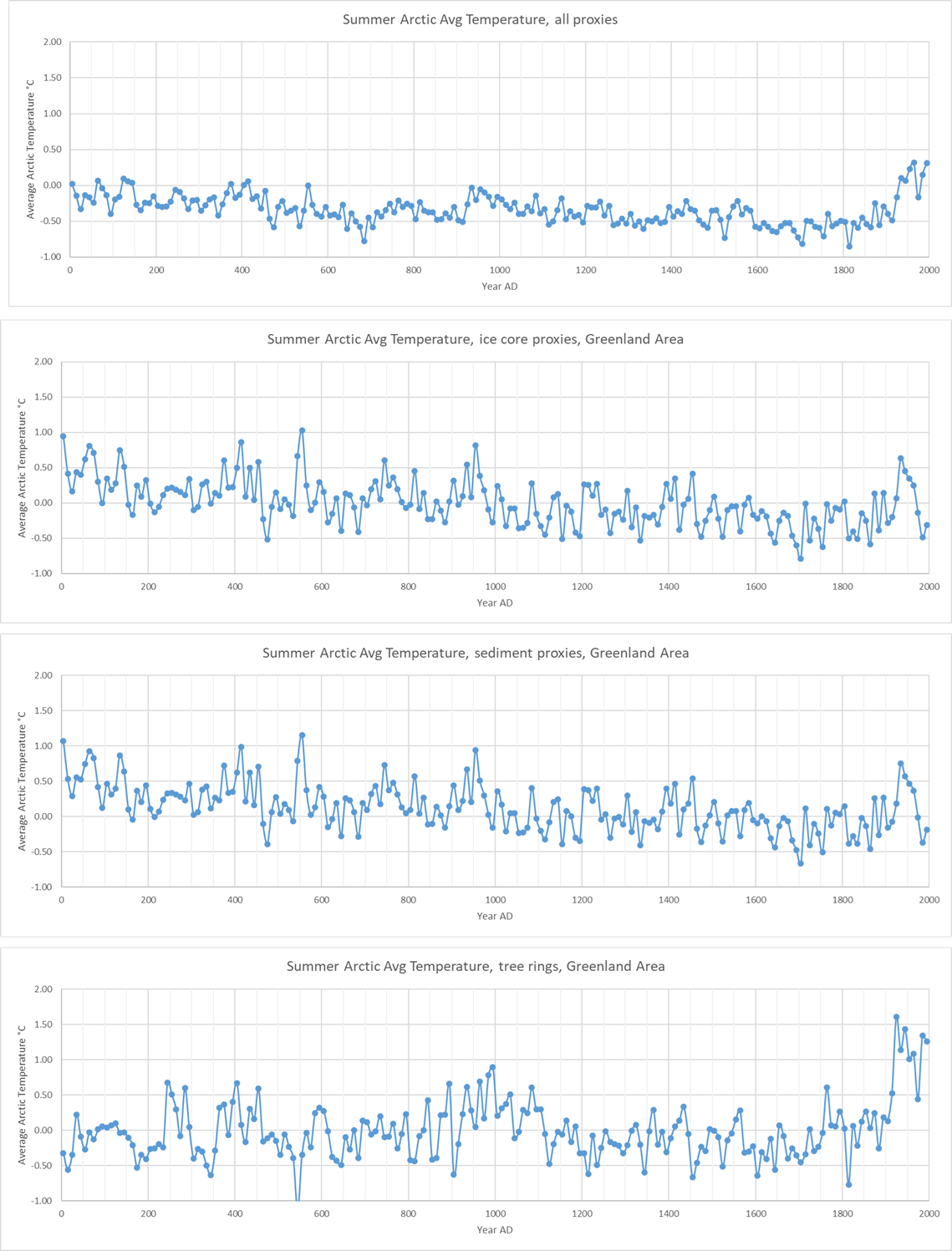
Figure 2. Kaufman’s combined proxies (top), ice core proxies (second from top), sediment proxies (third), and tree ring proxies (bottom). Source: (Kaufman et al., 2009) supplementary materials, corrected (see here).
The same modern discrepancy between the tree rings and the other proxies can be seen in Kaufman et al.’s figure 3A, reproduced as our figure 3 below.
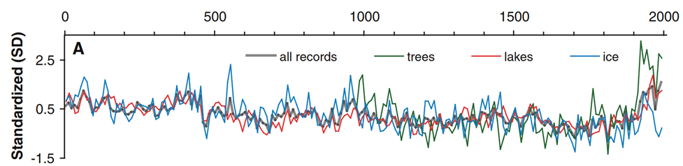
Figure 3. Kaufman et al. figure 3A. Arctic proxy overlay in standardized units. Source: (Kaufman et al., 2009). The tree ring proxies are shown in green and they diverge from the others.
There is general agreement that summer Arctic warming is driven by Earth’s orbital cycles, especially precession and obliquity (see figure 4). This post was inspired by a discussion on a previous post, the critical comment is here.
Figures 2 & 3 show that both recent Greenland area sediment and ice core proxies decline after ~1940, but the tree ring proxies mostly stay high. We will remember that the late Keith Briffa (Briffa et al., 1998b) warned us that tree ring proxies diverged from other proxies in 1998, he speculated that increasing CO2 probably had a lot do with this divergence. The divergence and Michael Mann’s attempt to hide the problem led to the now famous “hide the decline” (McIntyre, 2014) & (McIntyre, 2011) scandal after the 2009 CRU email dump. I have no answer for the divergence or the apparent time shifts between proxies in figures 2 & 3 but warn the reader that proxy temperatures are not temperatures that are comparable to thermometer readings we make today, they are just proxies and dates for the proxy readings are uncertain.
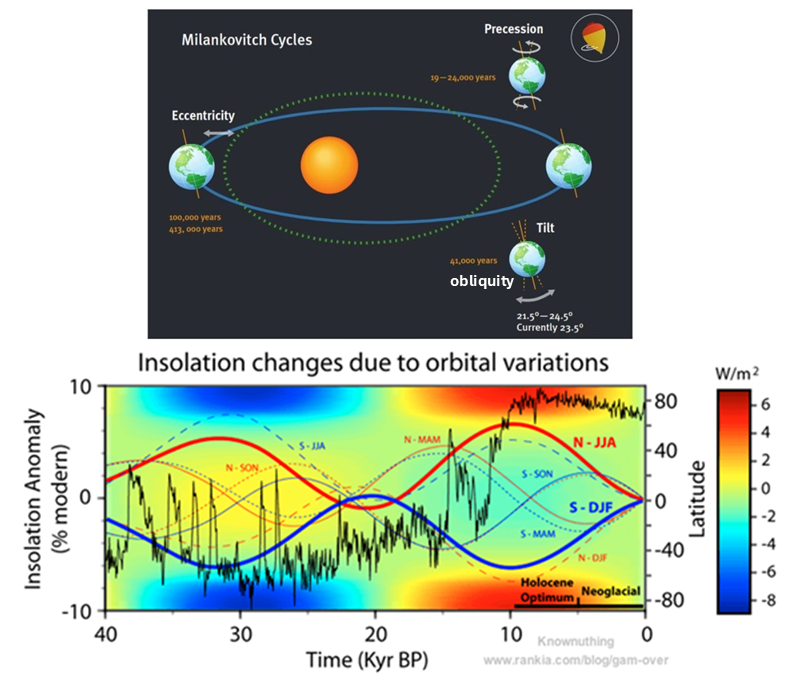
Figure 4. The top illustration, from (Haigh, 2011), shows the elements of the Milankovich orbital cycles, eccentricity, precession, and obliquity (or axial tilt). The bottom illustration from (Vinós, 2017) shows the climatic impact since 40,000 years BP.
The top illustration in figure 4 shows the elements of the Milankovitch cycles (Haigh, 2011). The seasonal curves in the bottom illustration (Vinós, 2017) show the impact of precession. The seasonal curves are labeled with the hemisphere (N or S) and the first letters of the months. The heavy curves are the summer months of the Northern Hemisphere (red) and the Southern Hemisphere (blue). The changes in insolation are represented by the background color (scale to the right in W/m2). The black curve shows the δ18O isotope changes from the NGRIP Greenland ice core analysis, a temperature proxy (Alley, 2000). The δ18O temperature proxy has no scale, but higher temperatures are up and lower temperatures down. The vertical scale is latitude, and the horizontal scale is time from 40,000 years ago to the present and zero on the background color scale is the insolation by latitude today.
The changes in the background color (insolation) in the bottom illustration in figure 4 are mostly due to changes in Earth’s orbital obliquity and are approximately symmetrical with regard to the hemispheres. The changes due to obliquity determine how much insolation reaches the poles versus the tropics. Precession on the other hand affects the seasonal distribution of solar energy, so as you can see, the end of the last glacial period at the beginning of the Holocene 11,700 years ago was when obliquity and precession were maximal in the Northern Hemisphere. Maximal precession means the difference in the Northern Hemisphere summer and winter was maximal, the total insolation by latitude remains about the same. Maximal obliquity means both poles receive the maximum insolation they will get, at the expense of the tropics.
Other interesting things to note in the lower part of figure 4 are that insolation barely changes throughout the Holocene in the tropics but changes a lot at the poles. The N-JJA (precession) curve looks a lot like the Makassar Strait and Greenland proxies in figure 1, notice the Holocene Climatic Optimum and Neoglacial labels in both figures 4 and 1.
Figure 5 shows the full Vinther and Rosenthal curves and relates them to historical events. Click on the figure or here to see at full resolution.
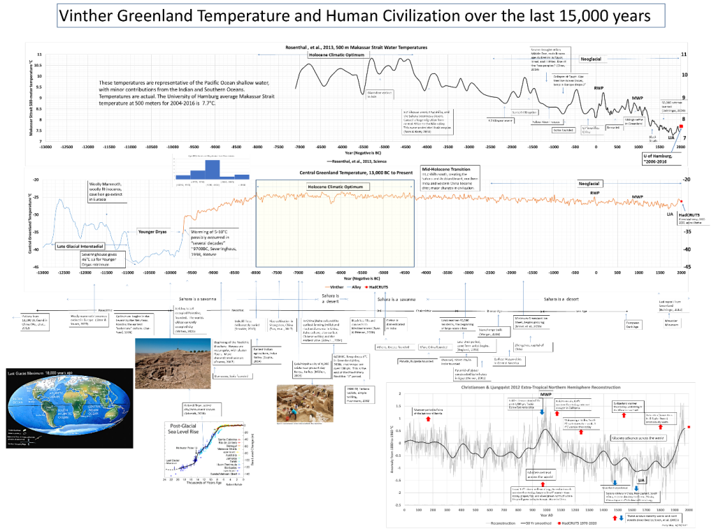
Figure 5. Vinther Greenland reconstruction (middle) and Rosenthal Makassar Strait reconstruction (top) compared to historical events. Click on the figure to see at full resolution. Source: Figure 3 here.
There are a large number of historical references in the timeline shown in Figure 5 and we will not explain all of them here, they are well documented in earlier posts here and here. We will just make the point that significant local climate changes are historical events that are often described in detail by the historians of the time and dated precisely. These historical descriptions can be more valuable than biological or ice core proxies.
As figure 4 shows, the Arctic received the maximum insolation at the beginning of the Holocene 9,700BC (Walker et al., 2009). This was also the time of the fastest change in Arctic temperature during the Holocene. Around 9,700BC Severinghaus et al. documented a 5-10°C warming event that took only a few decades, dwarfing the warming rate we observe today. The warming event is identified in the middle plot in figure 5. This warming event is so significant it is part of the official geological basis for the beginning of the Holocene Epoch (Walker et al., 2009).
The top plot in figure 5 shows the temperature of the 500-meter water in the Makassar Strait, which is representative of the North Pacific SST (Rosenthal et al., 2013). The present-day temperature in the Makassar Strait from the University of Hamburg (Gouretski, 2019) ocean temperature database is shown on this plot as a red box, it is well below the temperatures seen in the Medieval Warm Period (MWP) and the Roman Warm Period (RWP). In the middle plot of figure 5, the Vinther reconstruction (Vinther et al., 2009) is the orange line. The earlier blue line is the Alley reconstruction (Alley, 2000) spliced to it. The HadCRUT5 Greenland temperature average from 2000-2020 is plotted as a red box for comparison to the proxy temperature. The modern temperature in Greenland is roughly the same as the MWP temperature.
Discussion
There is considerable evidence that modern Arctic and Northern Hemisphere temperatures are well below the temperatures of 6,800-7,800 years ago. There is also a lot of evidence that the rate of temperature increase in 9,700BC was much faster than the increase we observe today. Comparing the rate of warming today when we have daily temperatures from all over the world to pre-industrial proxies is problematic. The high-quality Rosenthal and Vinther proxies have a resolution of about 20-years over the past 2000 years, so the modern averages that we compare them to in figure 5 cover 11 years (U of Hamburg) and 21 years (Greenland). It is much easier to reduce modern resolution for comparisons to the past than to try and increase proxy resolution. It is foolish to try and reconstruct global or hemispheric temperature records with proxies; they are very coarse and the averaging process used to make the reconstructions destroys the critical detail needed to determine a rate of warming.
Besides the rapid warming seen in these proxies around 9,700BC, there was also rapid warming around 6200BC, 40BC, and 800AD. Any of these periods could have warmed faster than today if they could be compared with the same coverage and accuracy.
Works Cited
Alley, R. B. (2000). The Younger Dryas cold interval as viewed from Central Greenland. Quaternary Science Reviews, 19, 213-226. Retrieved from http://klimarealistene.com/web-content/Bibliografi/Alley2000%20The%20Younger%20Dryas%20cold%20interval%20as%20viewed%20from%20central%20Greenland%20QSR.pdf
Briffa, K., Schweingruber, F., Jones, P., Osborn, T., & Vaganov, E. (1998b). Reduced Sensitivity of recent tree-growth to temperature at high latitudes. Nature, 678-682. Retrieved from https://www.nature.com/articles/35596
Gouretski, V. (2019). A New Global Ocean Hydrographic Climatology. Atmospheric and Oceanic Science Letters, 12(3), 226-229. Retrieved from https://www.tandfonline.com/doi/full/10.1080/16742834.2019.1588066
Haigh, J. (2011). Solar Influences on Climate. Imperial College, London. Retrieved from https://www.imperial.ac.uk/media/imperial-college/grantham-institute/public/publications/briefing-papers/Solar-Influences-on-Climate—Grantham-BP-5.pdf
Kaufman, D. S., Schneider, D. P., McKay, N. P., Ammann, C. M., Bradley, R. S., Briffa, K. R., . . . Vinther, B. M. (2009). Recent Warming Reverses Long-Term Arctic Cooling. Science, 325(5945). https://doi.org/10.1126/science.1173983
Lecavalier, B., Fisher, D., G.A. Milne, B., Vinther, L., Tarasov, P., Huybrechts, D., . . . Dyke, A. (2017). High Arctic Holocene temperature record from the Agassiz ice cap and Greenland ice sheet evolution. Proc. Natl. Acad. Sci. , 114(23), 5952-5957. https://doi.org/10.1073/pnas.1616287114
McIntyre, S. (2011, Dec. 1). Hide-the-Decline Plus. Retrieved from Climate Audit: https://climateaudit.org/2011/12/01/hide-the-decline-plus/
McIntyre, S. (2014, September 6). The Original Hide-the-Decline. Retrieved from Climate Audit: https://climateaudit.org/2014/09/06/the-original-hide-the-decline/
Rosenthal, Y., Linsley, B., & Oppo, D. (2013, November 1). Pacific Ocean Heat Content During the Past 10,000 years. Science. Retrieved from http://science.sciencemag.org/content/342/6158/617
Vinós, J. (2017, April 30). Nature Unbound III: Holocene climate variability (Part A). Retrieved from Climate Etc.: https://judithcurry.com/2017/04/30/nature-unbound-iii-holocene-climate-variability-part-a/
Vinther, B., Buchardt, S., Clausen, H., Dahl-Jensen, Johnsen, Fisher, . . . Svensson. (2009, September). Holocene thinning of the Greenland ice sheet. Nature, 461. Retrieved from https://www.nature.com/articles/nature08355
Walker, M., Johnsen, S., Rasmussen, U. O., Popp, T., Steffensen, J.-P., Gibbard, P., . . . Newnham, R. (2009). Formal definition and dating of the GSSP (Global Stratotype Section and Point) for the base of the Holocene using the Greenland NGRIP ice core,and selected auxiliary records. Journal Of Quaternary Science, 24, 3-17. https://doi.org/10.1002/jqs.1227
This article was published under the title ‘Holocene Warming’ on 4 February 2026 on Andy May Petrophysicist.

Andy May
Andy May is a retired petrophysicist and has published six books. He worked on oil, gas and CO2 fields in the USA, Argentina, Brazil, Indonesia, Thailand, China, UK North Sea, Canada, Mexico, Venezuela and Russia. He specialized in shale petrophysics, fractured reservoirs, wireline and core image interpretation, and capillary pressure analysis, besides conventional log analysis. His full resume is here: AndyMay

more news
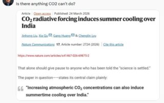
CO₂ Can Cause Cooling Too? Climate Models Say Yes (Sometimes)
As Dr. Matthew Wielicki dryly put it: “Is there anything CO₂ can’t do?” The study behind that remark claims that rising CO₂ levels may even lead to regional cooling under certain conditions—highlighting just how flexible—and uncertain—climate model outcomes can be.
Press release GWPF: Event Attribution Studies are “a blot on science”, says Ralph B. Alexander
Extreme weather attribution studies are based on flawed logic and misleading statistical practices, according to a new report by The Global Warming Policy Foundation (GWPF). Author Ralph B. Alexander argues that these studies, which link individual weather events to climate change, are driven more by political and legal agendas than by robust scientific evidence.
China’s Massive Coal-to-Liquids Expansion
In this article, Australian science writer Jo Nova examines China’s rapidly expanding coal-to-chemicals and coal-to-liquids industry. While much of the West focuses on phasing out fossil fuels, China is quietly transforming coal into fuels, plastics and fertilizers at massive scale—raising important questions about energy security and global climate policy.

