Climate Oscillations 12: The Causes & Significance
In this post we will examine the idea that ocean and atmospheric oscillations are random internal variability, except for volcanic eruptions and human emissions, at climatic time scales. This is a claim made by the IPCC when they renamed the Atlantic Multidecadal Oscillation (AMO) to the Atlantic Multidecadal Variability (AMV) and the PDO to PDV, and so on.

In this post we will examine the idea that ocean and atmospheric oscillations are random internal variability, except for volcanic eruptions and human emissions, at climatic time scales. This is a claim made by the IPCC when they renamed the Atlantic Multidecadal Oscillation (AMO) to the Atlantic Multidecadal Variability (AMV) and the PDO to PDV, and so on. AR6 (IPCC, 2021) explicitly states that the AMO (or AMV) and PDO (or PDV) are “unpredictable on time scales longer than a few years” (IPCC, 2021, p. 197). Their main reason for stating this and concluding that these oscillations are not influenced by external “forcings,” other than a small influence from humans and volcanic eruptions, is that they cannot model these oscillations, with the possible exceptions of the NAM and SAM (IPCC, 2021, pp. 113-115). This is, of course, a circular argument since the IPCC models have never been validated by predicting future climate accurately, and they also make some fundamental assumptions that simply aren’t true.
They also state that the variance over the observational records in the Pacific and Atlantic exhibit no significant changes (IPCC, 2021, p. 114). This is disputed in the peer-reviewed literature (Ghil, et al., 2002), (Scafetta, 2010), (Mantua, et al., 1997), and (Gray, et al., 2004). All the listed sources, and many others, found the AMO, PDO, ENSO, or the global mean surface temperature (GMST) oscillations to be statistically significant at the 95% level or higher, usually by comparing them to red or white noise.
While AR6 WGI (page 196) believes that the statistical significance of a change in climate (a signal to noise ratio greater than one) can be estimated with either observations or models, I believe only observations should be used. For the purposes of this post, a trend in observations will be tested versus a mean state with no definable time period, like white noise. That is, it covers all frequencies equally. We will also refer to “red noise,” which is like white noise, but has a higher content of lower frequencies and provides a stricter test than white noise (Ghil, et al., 2002).
At the other extreme is a perfect cycle that never varies in frequency. None of the oscillations are perfect cycles, the periods do vary. So, what we want is to measure how close the oscillation is to a perfect cycle and how far away it is from white or red noise. The statistical significance of observed oscillations varies considerably.
Finally, oscillations are inconsistent with anthropogenic greenhouse gas emissions as a dominant forcing of climate change. Greenhouse gas emissions do not oscillate; recently they have only increased with time. So, we will examine the relationship between solar and orbital cycles and the climate oscillations. As Scafetta and Bianchini (2022) have noted, there are some very interesting correlations between solar activity and planetary orbits, and climate changes on Earth.
Correlations with solar and planetary forces
Nicola Scafetta has identified strong climate oscillation frequencies with periods of ~9, ~20, and ~60 years that closely correspond to the orbital periods of the Moon, the rather complex movement of the Sun around the barycenter of the solar system, and the orbits of Jupiter, and Saturn (Scafetta, 2010). Frank Stefani has written about how the beat between the 22.14-year Hale solar cycle and the complex 19.86-year path of the Sun around the solar system barycenter can explain the ~193-year Suess-de Vries and two Gleissberg-type cycles close to 90 and 60 years. The computed periods turned out to be in amazing agreement with those derived from climate-related sediment data from Lake Lisan (see Figure 9 in Stefani et al., 2024) and may also explain the pacing of the Little Ice Age solar grand minima. The grand minima are plotted in figure 2 or the featured image of this post, also see (Stefani, et al., 2024).
The astronomical periods mentioned above all correlate, in phase, with observed climate oscillations on Earth. However, it is very unlikely that they are the only external influences affecting climate, probably volcanic eruptions, greenhouse gases, and true internal variability play a role as well. Further, our inability to measure climate change accurately plays a role in determining how Earth’s climate state changes with time. As we have seen in this series, the global mean surface temperature or GMST is a poor measure of the state of global or regional climate.
While internal variability may play a role in our observed oscillations, it is possible that gravitational forces and changes in solar output provide the pacing of the oscillations. Since all climate oscillations clearly influence the others through a mechanism named “teleconnections,” if the pacing of a few of the oscillations is driven by gravity, tides, and solar variability, then the pacing can be transmitted to all of them.
Major teleconnection patterns are large scale Rossby waves that can last for months and sometimes persist around the entire planet. They define the “waviness” of the jet streams and thus the weather in the mid-latitudes, especially in winter. They vary on all time scales, daily, monthly, annually, and decadally. The illustration in figure 1, from climate.gov, shows a Rossby planetary wave. If you’ve read the previous Climate Oscillation posts (see the full list at the bottom of this post) you will recognize how closely related Rossby waves are to the oscillation patterns I have been writing about.
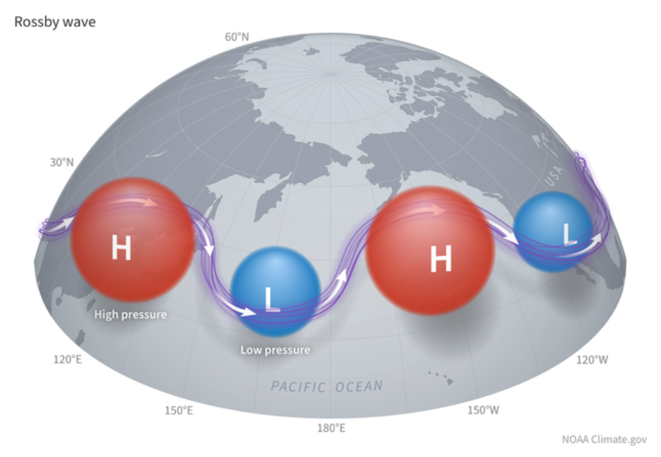
Figure 1. An illustration of a Rossby wave from climate.gov. The waves create alternating high and low pressure regions.
These regions can move over long periods of time and the movement can be seen in many climate oscillations.
Rossby waves can create a sort of domino effect through all major hemispheric oscillations as described by Marcia Wyatt’s “stadium wave” hypothesis (Wyatt, et al., 2012a) and (Wyatt & Curry, 2014). Unfortunately, the fact that multiple extraterrestrial forces are contributing to affect our climate patterns and Rossby waves are not static, and they vary in sometimes unpredictable ways, the resulting climate oscillations vary in period and strength as we have seen in the earlier posts of this series.
If we define “global climate change” as the observed changes in HadCRUT5 or BEST global mean surface temperature (GMST) as the IPCC does, then the oscillations that correlate best are the AMO and the global mean sea surface temperature (SST) as shown in figure 2. None of the other oscillations correlate well with GMST.
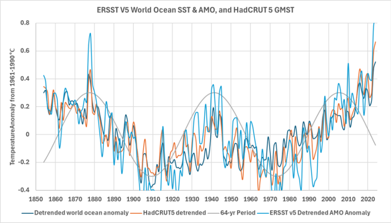
Figure 2. Detrended HadCRUT5 compared to the detrended world ocean mean SST and the AMO.
In figure 2, the gray curve is a 64-year cosine function. It fits the 20th century data but departs significantly around 2005 and before 1878. The early departure could be due to poor data, the 19th century temperature data is very bad, see figure 11 in (Kennedy, et al., 2011b & 2011). Data quality problems still exist today, but are much less of a factor and the departure after 2005 is likely real and could be caused by any combination of the of the two following factors:
- Human-emitted greenhouse gases.
- The full AMO/world SST/GMST period is longer and/or more complex than we can see with only 170 years of data.
It is probably a combination of the two. As discussed by Scafetta and Stefani, climate, orbital, and solar cycles are known to exist that are longer than 170 years. The fact that I had to detrend all the records shown in figure 2 testifies to that. It is also noteworthy that the ENSO ONI trend since 2005 is trending down; as shown in the last post. So is the current PDO trend. All the notable oscillations are not synchronized, teleconnections or not, climate change is not simple. The trends in figure 2 result from complex combinations of gravitational forces and teleconnections (Scafetta, 2010), (Ghil, et al., 2002), and (Stefani, et al., 2021).
60-70-year oscillations
In the twentieth century the AMO appears to have a period of about ~64 years, ±5 years (Wyatt, et al., 2012). The same ~64-year period fits HadCRUT5 and the global average SST record as shown in figure 2. Scafetta illustrates a similar ~61-year oscillation in GMST and highlights its match to the Sun’s speed around the center of mass of the solar system (SCMSS), as shown in figure 10 in Scafetta (2010). Of the oscillations studied in this series, the AMO, global SST mean, and HadCRUT5 are unique in that they do not have a strong frequency content in the 5–25-year bands (Gray, et al., 2004).
Marcia Wyatt’s “stadium wave” hypothesis shows that a suite of global and regional climate indicators vary over roughly the same 64-year period (Wyatt, 2020), (Wyatt, et al., 2012a), and (Wyatt & Curry, 2014). Although the climate indicators have about the same period, they are offset from one another in time. Using data from the 20th century, the AMO, global SST, and HadCRUT5 have lows in 1904-1911 and 1972-1976.
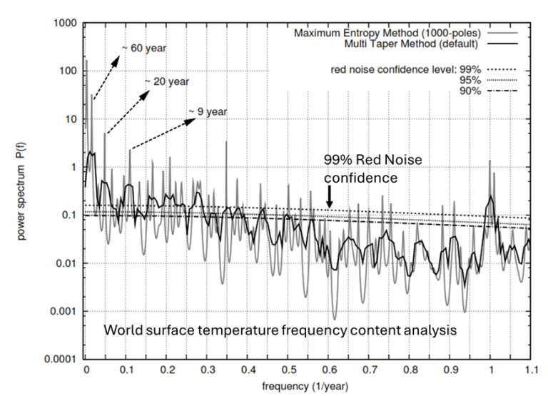
Figure 3. Frequency analysis of the HadCRUT3 GMST record from 1850-2009. Source: (Scafetta, 2010).
Nicola Scafetta did the frequency analysis of the HadCRUT3 global mean surface temperature shown in figure 3. It shows that the roughly ~60-year periodicity in GMST is present in the record with a confidence of 99% when compared to red noise.
As we can see in figure 2, the ~64-year period does seem to have broken down over the past 20 years. Scafetta provides a good summary of the evidence for a ~60-year global climate oscillation and establishes that this period is significant at the 99% level. What we might be seeing at the end of the record in figure 2 is the influence of CO2, the strong 2016 El Niño, the Hunga Tonga volcanic eruption, and a smaller natural temperature maximum that follows the 60-year maximum by ~20 years (ie. 2020-25) that was predicted in Scafetta (2010) in his figure 10.
As Scafetta and Bianchini note, the ~60-year cycle has been known since antiquity, Johannes Kepler mentioned it in his writings in 1606. Scafetta also provides a list of several climate and environmental series that have a strong ~60-year period component, including G. Bulloides abundance in the Caribbean Sea since 1650, berylium-10 and carbon-14 records, as well as in Earth’s angular velocity and magnetic field (Scafetta, 2010). The ~60-year cycle may be related to the orbits of Jupiter and Saturn (Scafetta & Bianchini, 2022).
The specific mechanism behind the ~60- or ~64-year oscillation is unknown. However, Scafetta (2021) has proposed a reason the modern oscillation is 64 years, whereas the historical cycle is closer to 60 years. Using data from the CMIP5 models, he removed the anthropogenic greenhouse gas (using an ECS of 1.5°C/2xCO2) and volcanic forcings and the oscillation moved from 64 years to 60. He concluded that the natural oscillation is about 60 years. His analysis shows that the CMIP climate models are missing an important natural climate change forcing. That is, the changes in insolation due to changes in the Sun, which, in turn, are due to planetary orbital patterns. Once the solar changes are incorporated into the model the computed ECS is cut in half to about 1.5°C/2xCO2, which fits the ECS values computed from observations.
20-30-year oscillations
Nathan Mantua and colleagues (Mantua, et al., 1997) identified 20th century “climate shifts” in the PDO in 1925, 1947, and 1977, which results in a major multidecadal climate oscillation of 22 to 30 years. We identified two additional possible PDO shifts in 1898 and 1997 in post 8 of this series. The average difference is around 25 years. A 25-year period is shown with a 5-year-smoothed PDO in figure 4.
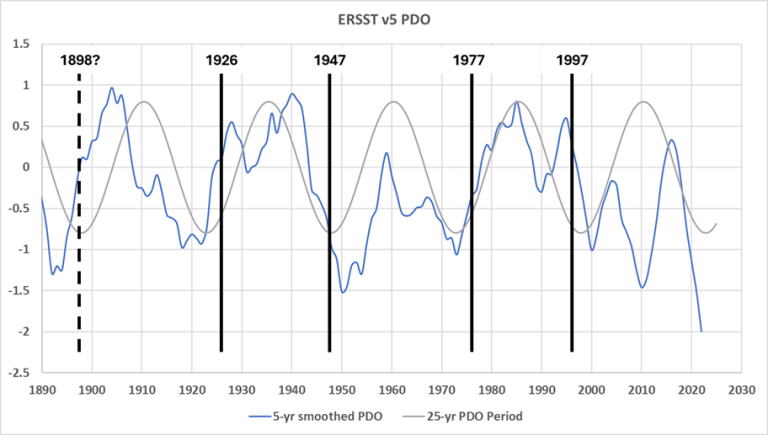
Figure 4. ERSST v5 PDO, the recognized Pacific climate shifts are noted
on the plot as well as the more speculative 1898 and 1997 possible shifts.
Solar and orbital oscillations of ~20- and ~30-years, that correlate with climate oscillations like the PDO, have been observed (Scafetta, 2014). These solar cycles are near the PDO oscillation shown in figure 4.
The 2-, 5-, 9-, and 11-year oscillations
Frank Stefani and colleagues and Nicola Scafetta and Antonio Bianchini (2022) make convincing cases that the Schwabe 11.07-year solar cycle is built from Jupiter and Saturn (9.93 years), Jupiter alone (11.86 years), and/or the periodic linear alignment of Earth, Venus, and Jupiter. According to Nicola Scafetta, the fact that the 11-year Schwabe solar cycle is related to the “influences of Venus, Earth, Jupiter and Saturn,” was proposed by Johann Rudolph Wolf as early as 1859 (Scafetta & Bianchini, 2022).
There is a statistically strong period of 9 to 9.2 years in most temperature records, and this periodicity matches half the lunar-solar orbital cycle, thus the periodicity matches the pattern of strong lunar tides on Earth and the periodicity is evident in ocean records (Scafetta, 2010). Besides lunar tides, evidence that a Jupiter-type planet can induce a 9-year activity cycle in any star has been known for some time (Scafetta, 2014).
The two dominant periods in the ENSO SOI (similar to the ONI discussed in post 11) are 2.4 and 5.5 years. Both periods are significant at the 99% level (Ghil, et al., 2002). GMST also shows a significant period of about 5.5 years. The speed of the sun around the center of mass of the solar system also has a significant period of 5.5 years (Scafetta, 2010).
The QBO (the Quasi-Biennial Oscillation) has an average period of 28 months or 2.3 years. This is a stratospheric wind that circles the globe in the tropics. It changes direction from easterly to westerly about every 28 months and this periodic change is called the QBO. The QBO is important for seasonal weather forecasting, it exerts a considerable effect on stratospheric ozone, and it influences how the sun affects Earth’s climate (see the discussion here). Exactly how solar activity affects the QBO is unknown. Interestingly, though, Frank Stefani explains the solar pendant of the QBO in terms of the 1.723-year beat period of the two-planet tidal forcings from Venus, Earth, and Jupiter. This number agrees strikingly with the observed period of sporadic relativistic solar particles detected at the Earth’s surface by cosmic ray detectors. These solar particle events (called “Ground Level Enhancement” events) occur preferentially in the positive phase of the QBO and have a beat period of 1.73-year (Herrera, et al., 2018) or 1.724 years (Stefani, et al., 2025).
Discussion
The causes of climate change are a complex mixture of many natural cycles, perhaps some human activities, and natural variability. This is far more sensible than “CO2 done it,” which is still what many believe today. Exactly how climate change works is still unknown, but fortunately much more research into natural causes is being done today than in the past. This series was meant to bring my readers up to date on the quest. One thing is for sure; climate is a regional long-term trend, it is not global mean surface temperature!
The oscillations described in this series are not internal variability with a little push here and there from manmade greenhouse gas emissions or volcanic eruptions, as proposed by Michael Mann (2021). They are too regular, and many can be traced back thousands of years through proxies. They also correlate extremely well with environmental changes that can be traced into the past (Ebbesmeyer, et al., 1990) and (Scafetta, 2010). Finally, they affect one another through teleconnections that themselves have statistically significant decadal to multidecadal oscillations.
The strong climate oscillations correlate quite well with planetary motions that have major periods of about 11, 12, 15, 20-22, 30, and 61 years. These cycles are related to the orbital patterns of Jupiter, Saturn, and Earth (Scafetta, 2010). The 11- and 22-year periods are also the well-known Schwabe and Hale cycles. The common 9.1-year cycle is related to the long-term orbital motion of the Moon.
The roughly 60-year oscillation that is so prominent in many records is likely the most powerful, it can be seen in the length-of-day (see post 4), auroral records (Scafetta, 2012c), berylium-10 and carbon-14 records, as well as global climate oscillations and in the stadium wave. The exact mechanism of how it affects climate is unknown. The second most powerful oscillation is the 20-22-year oscillation probably powered by the previously mentioned solar path around the solar system barycenter and the 22-year Hale solar cycle. Besides the shorter solar/climate oscillations mentioned in this post, there are longer oscillations or cycles that can be seen in climate proxies. Some of the most important are discussed here.
As mentioned previously in this series, the observed climate oscillations are not reproduced well in the CMIP climate models. Scafetta provides a good analysis of the model problems in (Scafetta, 2012c).
The climate oscillations described in this series are real and they do correlate with planetary movements and known solar cycles. It is reasonable to assume that the planetary orbits and solar cycles are helping to pace the oscillations and/or cause them. Proxies have shown that most of the oscillations can be traced back in time hundreds or thousands of years with some confidence, thus the inability of the CMIP climate models to reproduce them destroys the models’ credibility. The attempts by the IPCC, and others, to claim the oscillations are “natural variability” and not forced or paced by the Sun and planetary orbits, makes no sense.
Climate change and climate itself is a complex, poorly understood, dance of regional oscillations around the world. The dance is choreographed by teleconnections that themselves vary decadally. Each oscillation and teleconnection influences the others to some degree as alluded to in Marcia Wyatt’s papers. On a global scale, they dance their way through a roughly 64-year global oscillation. This is the way the world has worked for millions of years, and we will never be able to understand how humans influence climate until we understand exactly how these natural oscillations work. Proclaiming that we control the climate without first understanding how nature works is a fool’s errand.
This post has been reviewed by Nicola Scafetta and Frank Stefani who suggested some very useful corrections and additions. I am indebted to them, but any remaining errors are mine alone.
Download the bibliography here.

Andy May
This article was published on August 5, 2025, by Andy May on his website andymaypetrophysicist.com.
Andy May is a retired petrophysicist and has published six books. He worked on oil, gas and CO2 fields in the USA, Argentina, Brazil, Indonesia, Thailand, China, UK North Sea, Canada, Mexico, Venezuela and Russia. He specialized in shale petrophysics, fractured reservoirs, wireline and core image interpretation, and capillary pressure analysis, besides conventional log analysis. His full resume is here: AndyMay

Previous posts in this series on Andy May Petrophysicist:
Climate Oscillations 1: The Regression
Climate Oscillations 2: The Western Hemisphere Warm Pool (WHWP)
Climate Oscillations 3: Northern Hemisphere Sea Ice Area
Climate Oscillations 4: The Length of Day (LOD)
Climate Oscillations 6: Atlantic Meridional Model
Climate Oscillations 7: The Pacific mean SST
Climate Oscillations 8: The NPI and PDO
Climate Oscillations 9: Arctic & North Atlantic Oscillations
Climate Oscillations 10: Aleutian Low – Beaufort Sea Anticyclone (ALBSA)

more news

The Strait of Hormuz’s Bitter Lesson for the European Union
In May 2023, Ursula von der Leyen, President of the European Commission, declared that the fossil-fuel-based growth model is “simply obsolete.” The partial blockade of the Strait of Hormuz starkly exposes the irony of that statement, says Samuel Furfari.

“Climate Policy Ignores Nature” – Interview with New WCD Signatory Enrique Ortega
Spanish geologist and new World Climate Declaration signatory Enrique Ortega brings decades of experience in earth sciences to the climate debate, emphasizing the importance of geological history in understanding present-day climate change.

In a Warming World, Rising Cold Deaths Outnumber Heat Deaths 12 to 1
A new paper shows that in the USA, cold weather is a much larger contributor to mortality than heat, and that social vulnerability plays a major role in determining outcomes.

