“Consensus” scientists do not believe that solar variability, internal climate variability (in this model simplified to the ~67-year stadium wave), or volcanism influence net global warming or climate change since 1750, yet considerable evidence exists that these factors have an impact. I’ve previously built a model of the HadCRUT5 global average temperature (see here) from seven known climate and solar cycles using multiple regression and was reasonably successful.

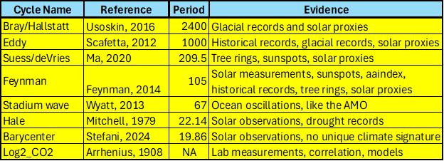
In this attempt, I utilize the six best documented solar/climate cycles in listed Table 1 and the stadium wave climate-only interior variability cycle to create a multiple regression model of HadCRUT5.

Table 1. Solar and climate proxies and measurements used in this model.

When using many series to build a multiple regression model one is always confronted with von Neuman’s joke that with four arbitrary parameters he can fit an elephant. Further, all these series are serially correlated, which weakens the computed statistics of the resulting fit, such as R². However, none of these series are “arbitrary parameters.” Except for the stadium wave and Log2_CO₂ they are observed solar and climate cycles that share the same period and are in phase with one another. All are well supported with multiple lines of evidence. Thus, they are quite constrained and not arbitrary.

While they are not arbitrary in the von Neuman sense, they are not independent of one another. Probably the solar dynamo is behind all of them, but the mechanism Sun → climate is not understood for any of them except possibly for the Hale Cycle and the Barycenter. The solar dynamo is quite complex, especially in the longer term.

The stadium wave has no associated solar cycle and seems to be wholly internal variability, it has a period of roughly 67 years and correlates well with global average temperature (May & Crok, 2024). Internal climate variability is poorly understood and simply choosing the stadium wave to represent it is probably a vast oversimplification, but it is the best I can do. For a good up-to-date discussion of the components of internal variability I recommend Marcia Wyatt’s excellent report on circulation patterns (Wyatt M. , Circulation Patterns: Atmospheric and Oceanic, 2020). The report is paywalled, but a slightly different earlier version of the same report can be downloaded here.

The whole point of including the stadium wave is to account for the variable lag in emitting received solar radiation to space. Most solar radiation is received in the tropics, more than they can emit to space. As a result, some of the radiation received in the tropics must be transported to higher latitudes which emit more energy than they receive, especially in the winter months. Atmospheric and ocean circulation patterns change the timing of this tropics-to-pole energy transfer. A longer time to emit absorbed solar energy causes the planet to warm and a shorter time causes it to cool. Earth is never in thermal equilibrium except briefly by coincidence and the thermal energy residence time in the ocean/atmosphere climate system is constantly changing but seems to have roughly a 67-year cycle. The 67-year cycle overlies a longer secular trend of change, that longer trend could be due to solar cycles or CO₂ or both. See figure 2 in May & Crok as an example.

There are no measurements from space or in the atmosphere that support the hypothesis that additional CO₂ (man-made or otherwise) will cause global warming, but there are lab measurements, correlations, and climate models that support the hypothesis. CO₂ has some effect, but how much is anyone’s guess at this point. We try and use multiple regression to derive a value below.

Critical Solar and Cycles

In this section we briefly describe each of the six well documented solar cycles listed in Table 1 that have a demonstrated impact on Earth’s climate and provide references for them.

Bray/Hallstatt Cycle

Roger Bray used glacial advance and retreat records to identify an approximately 2400-year climate cycle originally called the “Hallstatt” cycle (Bray, 1968). Although originally discovered by its effect on Earth’s climate there is an associated solar cycle that is in phase with the climate cycle and has the same period as discussed here. A more technical discussion of the solar Bray/Hallstatt Cycle is presented by Ilya Usoskin et al. here (Usoskin, Gallet, Lopes, Kovaltsov, & Hulot, 2016). A low in the Bray Cycle played a role in creating the very cold period from about 1650-1715AD during the Little Ice Age.

Eddy Cycle

The roughly 1000-year Eddy Cycle was named by José A. Abreu and colleagues (Abreu, Beer, & Ferriz-Mas, 2010). They note that John Eddy identified and documented periods of very low solar activity that corresponded with colder climates on Earth, like the Little Ice Age (Eddy, 1976). The 1000-year climate cycle can be seen by combining the Medieval Warm Period (roughly 800 to 1250AD with the Little Ice Age (roughly 1300-1850AD). Solar proxies find a 1000-year solar cycle that is in phase with the climate cycle as pointed out by John Eddy, see figure 5 in (Eddy, 1976). More on the Eddy Cycle can be seen in Javier Vinós’ book (Vinós, 2022), Chapter 8, page 123 here. The powerful Bray Cycle and the Eddy Cycle both had lows between 1470 and 1680 which undoubtably contributed to that extremely cold time during the Little Ice Age. For more on the Little Ice Age see (May & Crok, 2024) and here.

De Vries Cycle

The De Vries Cycle is also often called the Suess Cycle after Hans Suess (Suess, 1955) and (Sonett & Suess, 1984). Like most cycles it was first discovered in climate proxies, especially tree ring records, and it has a period of 193-209 years. The matching solar cycle is probably related to a beat period between the fundamental Hale Solar Cycle and the rosette-like motion of the Sun around the solar system barycenter (Stefani, Horstmann, Klevs, Mamatsashvili, & Weier, 2023).

Feynman Cycle

It was always recognized that some sort of solar cycle existed with a period between 50 and 150 years and the mysterious poorly defined cycle was usually called the Gleissberg Cycle. Meanwhile a climate cycle with a length of about 100 years was also observed. Eventually Joan Feynman nailed down what is now called the ~100-year Feynman Solar Cycle in 2014 (Vinós, 2022, p. 129) and (Feynman & Ruzmaikin, 2014). We use a period of 105 years for the Feynman Cycle. The Feynman climate and solar cycles have the same period and are in phase.

Hale Cycle

The 22.14-year Hale Cycle is a very prominent solar cycle that is formed by a 22-year fundamental period of solar magnetic activity. It encapsulates two solar cycles that are marked by reversals of the solar magnetic field. Thus, one Hale cycle sees a reversal of the magnetic field and then a return to the original polarity. The Hale Cycle is closely related to the 22-year southwestern U.S. drought cycle (Mitchell, Stockton, & Meko, 1979).

Solar Barycenter rosette

The Sun tracks a complicated rosette-like motion about the solar system barycenter that takes 19.86 years (Stefani, Horstmann, Klevs, Mamatsashvili, & Weier, 2023). Any climate cycle associated with this is buried, or possibly shared, with the Hale Cycle.

Other Natural Climate Cycles

Stadium Wave

What we call the Stadium Wave Cycle or oscillation is a very strong global climate cycle that has a period of about 67 years (Wyatt & Curry, Role for Eurasian Arctic shelf sea ice in a secularly varying hemispheric climate signal during the 20th century, 2014) and (Wyatt M. G., 2012c). It is composed of many climate oscillations that propagate in an organized fashion across the Northern Hemisphere and affect the climate of much of the globe. It is not clear if this oscillation is related to a solar cycle.

CO₂

CO₂ as a factor that influences climate was first properly described by Svante Arrhenius in his book Worlds in the Making (Arrhenius S. , 1908), but he also discusses it in an earlier paper (Arrhenius S. , 1896). Even before Arrhenius’ attempt to quantify the atmospheric CO₂ concentration’s impact on the climate, the idea that CO₂ can affect Earth’s climate was also discussed, although in a less quantitative way, by Fourier (Fourier, 1824), Tyndall (Tyndall J. , 1861) and (Tyndall J. , 1859), and Langley (Langley, 1884). None of these earlier writers suggested that atmospheric CO₂ concentration “controlled the climate,” as the IPCC proposes in AR6 and previous reports (IPCC, 2021, p. 179), (Lacis, Hansen, Russell, Oinas, & Jonas, 2013), and (Lacis, Schmidt, Rind, & Ruedy, 2010). They also did not believe that human CO₂ and other greenhouse gas emissions were responsible for almost all the warming Earth has experienced since 1750 as claimed by the IPCC in AR6, page 961, figure 7.7.

None-the-less, CO₂ and other greenhouse gas concentrations probably do influence the average atmospheric temperature, however the idea that they somehow “control” the global average surface temperature and climate change is highly doubtful.

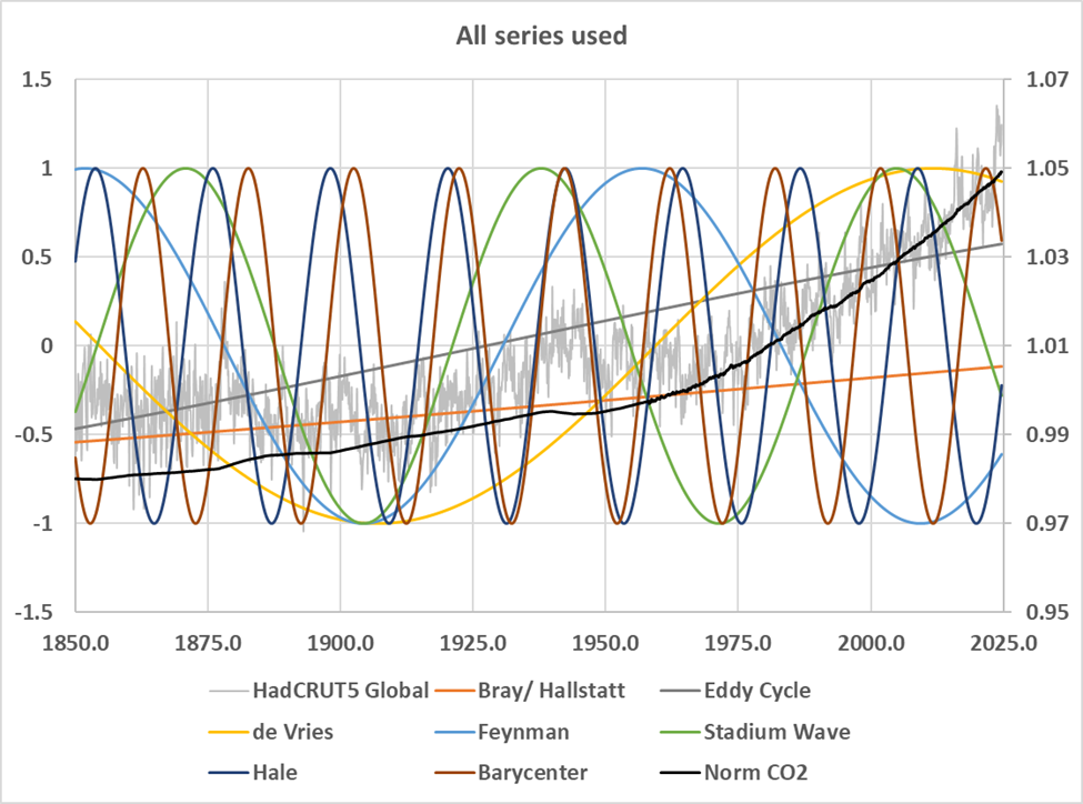
Figure 1 is a plot of all the series discussed in this post.

Figure 1. The time series discussed in this post.

Discussion

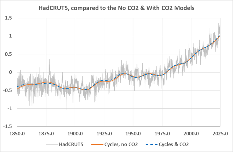
If we use the top seven series listed in table one, that is everything but CO₂, and regress against HadCRUT5 we get the result shown in orange in figure 2. If we then regress everything, including CO₂, we get the blue dashed line in figure 2. The two lines are nearly identical.

Figure 2. The faint gray line is HadCRUT5, the orange line is a regression against it using only the solar and climate cycles, the blue dashed line uses the same cycles, but adds the Log, base 2, of CO₂.

Now, that is interesting! The fit with the climate/solar cycles only and the fit with CO₂ and the same cycles are nearly identical. We need more information to make sense of this. Below are the statistics of the two regressions.

Table 2. Statistics of the regression with all the solar/climate cycles, but no CO₂. Adjusted R² = 0.8523.

Table 2 shows the statistics of the regression with no CO₂. The derived coefficients are on the left, and the mean and standard deviation of each series are shown and then the normalized coefficients. We can see that the Bray and Eddy Cycles are the most important series, and they slightly oppose one another since they have different signs. All the “P” values are good. The standard errors for the Bray and Eddy Cycles are a bit high, but that may be because their coefficients have opposite signs.

In Table 3 we show the statistics for the regression that contains CO₂.

Table 3. The regression statistics when CO₂ is added. Adjusted R² = 0.8548

Table 3 contains a lot of new and valuable information. In Table 2 the normalized coefficients show that the Bray and Eddy Cycles dominated the regression, but in Table 3 it is CO₂, by a long way and the P values for both Bray and Eddy have become unacceptable. CO₂ has essentially replaced the strong Bray and Eddy Cycles and knocked them out. Removing those two cycles results in the De Vries cycle becoming unacceptable with a P value of 0.37, so I also removed it, and the result is shown in Table 4.

Table 4. The regression statistics when CO₂ is added. Adjusted R² = 0.8548

In Table 4 all the P values are acceptable and CO₂ dominates the regression. For all practical purposes the adjusted R² from all three regressions are identical at about 0.85. The “adjusted R²” is corrected for the number of predictor variables and the number of observations. In all these cases the regular R² is nearly identical to the adjusted R².

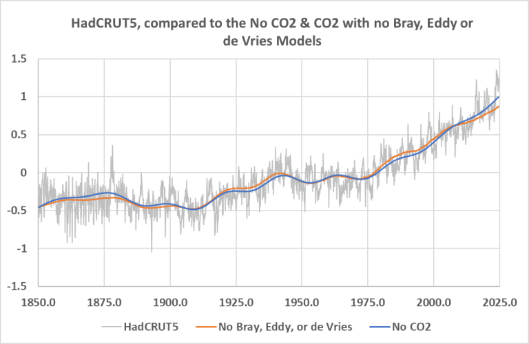
Figure 3 compares the no CO₂ case to the case described in Table 4.

Figure 3. Comparing the all-cycles/no CO₂ regression in blue to the CO₂ and no Bray, Eddy or de Vries cycles in orange. Statistics for the orange regression are given in Table 4.

Conclusions

As usual in climate science (and statistical analysis) you can take away whatever you like from this analysis. Statistics and climate science are similar in this way, you can always generate a lot of discussion around either of them and still know nothing.

CO₂ makes no difference if all the climate/solar cycles are used, but CO₂ can replace the most powerful Bray, Eddy, and de Vries solar/climate cycles. Objectively, one could point out that solar cycles (including the Milankovitch cycles) have driven climate change as far back as we can trace them with proxies and historical records, so why would we think CO₂ is driving climate if adding it to the regression makes no difference?

On the other hand, CO₂ can replace the very powerful Bray, Eddy, and de Vries cycles and get the same result. As usual, this analysis just shows we have no clue what drives climate change, but isn’t that what we’ve been saying all this time?

One can look at these plots and statistics and conclude that the impact of CO₂ on climate is zero, or they can conclude it is 100%. This study is inconclusive by itself. However, it also shows that well-known solar cycles, combined with internal variability can explain recent global warming; CO₂ is not required to explain it.

As with all purely statistical studies, this regression model is unsuitable to use in forecasting or hindcasting, the large coefficients in tables 2 to 4 show that. The value of the study is only to demonstrate that CO₂ is not necessary to explain recent warming.

This post looks at the problem “does CO₂ control global warming?” from a statistical perspective. To see how experts in climate science look at it from an atmospheric physics perspective it is worth reviewing the excellent 2014 American Physical Society workshop on climate change hosted by Steve Koonin. It is discussed and summarized here.

This post is the result of many email conversations with Charlie May, who contributed substantially to the ideas and models presented herein.

Download the bibliography here

Download the Regression statistics here.

Download the data used and the plots here.