To read this post in German see here, translation by Christian Freuer.
The IPCC and the climate “consensus” believe that essentially all warming since 1750 is due to man’s emissions of CO2 and other greenhouse gases as shown in figure 1 here or in (IPCC, 2021, p. 961). This has led to a 45-year search for the value of the Equilibrium Climate Sensitivity to the doubling of CO2 (“ECS” in °C per 2xCO2). Yet, after spending 45 years trying to calculate the sensitivity of climate to man-made greenhouse gases, the “consensus” has been unable to narrow the uncertainty in their estimates and, if anything, the climate model uncertainty is now larger than in earlier reports(IPCC, 2021, p. 927). It is now clear, at least to me, that modern climate models make many critical assumptions that are poorly supported and sometimes conflict with observations. This is an attempt to explain some of these problems and how they developed over time. It is long past time for the “consensus” to stop ignoring the obvious weaknesses in their 60-year old conceptual model of climate.
The Early Models
Syukuro Manabe built the first general circulation climate model with several colleagues in the 1960s (Manabe & Bryan, 1969) and (Manabe & Wetherald, 1967). He started with a one-dimensional radiative equilibrium model of horizontally averaged temperature but realized that the troposphere was not in radiative equilibrium because of convection. The lower atmosphere is nearly opaque to most surface emitted infrared radiation or Outgoing Longwave Radiation (OLR) because of greenhouse gases. As a result, Earth’s surface is not cooled much by emitting radiation but instead mostly by the evaporation of surface water that carries surface heat into the atmosphere as latent heat inside water vapor. Water vapor is less dense than dry air, so it rises. Once the water vapor is high enough, it cools as the surrounding air pressure drops allowing air parcels to expand, causing the water vapor to condense which releases its latent heat. If this is done at a high enough altitude, some of the latent heat can make it to space as radiation or make it to surrounding greenhouse gas molecules higher in the atmosphere. The rest of the released heat simply warms the neighborhood. This process is called the “moist adiabat.”
This process works because temperature declines with altitude in the troposphere according to a ”lapse rate.” The lapse rate varies a lot around the Earth, but the average gradient stays fairly constant at about 5.08 °C/km (Benestad, 2017, pp. 24-26, supp. mat.). The lapse rate is usually given as a positive number, but it is the decrease in temperature with height. The value we most often hear is 6.5 °C/km, even though the true average rate is lower. The actual lapse rate at any given location and time of day varies a lot, it also varies with humidity, and by season. The lapse rate can be negative, a state called a temperature inversion.
For Manabe’s early models he added a constraint on the lapse rate so that it could not rise above a fixed and assumed value so the model correctly predicted the position of the tropopause. The tropopause is the altitude where the temperature gradient stops being controlled by convection. Above the tropopause, the atmosphere is closer to thermal equilibrium and temperature rises with altitude. In Manabe’s early models the tropospheric lapse rate was assumed to be linear and fixed (Held & Soden, 2000).
Manabe also assumed fixed relative humidity and fixed cloud cover. As Held writes, it is an oversimplification to assume the lapse rate does not change with temperature, but it was a convenient assumption (Held & Soden, 2000). The assumption of fixed relative humidity results in an implausibly high sensitivity to CO2. In the tropics the temperature profile is similar to a moist adiabat (described above). The condensation of water vapor at altitude is the process that forms clouds (Held & Soden, 2000). Climate models have a very tough time reproducing the tropospheric temperature profile in the critical tropical regions because they predict too much warming due to greenhouse gases (IPCC, 2021, p. 443).
In the higher latitudes the moist adiabat does not work, since sensible and latent heat horizontal transport by mid- and high-latitude storms play a significant role in the overall climate (Held & Soden, 2000).
The Fixed Lapse Rate Assumption
A fixed lapse rate means that the global average emission temperature never changes, thus the outgoing longwave radiation doesn’t change, except briefly as the surface temperature changes. A common description of the greenhouse effect (GHE) includes a diagram of the lapse rate shown in figure 1 from (Held & Soden, 2000).
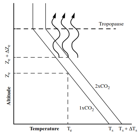
Figure 1. Held and Soden’s greenhouse effect model. Notice the effective emission temperature does not change, thus the amount of OLR does not change.
Figure 1 illustrates what doubling CO2 does with a fixed and linear lapse rate in Held’s simplified model. The additional CO2 warms the lower atmosphere with additional back-radiation, then the assumption of a fixed lapse rate kicks in, forcing the emission level up to a higher altitude, which means it has a lower temperature, causing it to emit less to space. Since it is emitting less radiation (aka “heat”), after a short period, the new emission level warms to the temperature of the old emission level and the effective emission temperature remains unchanged, as does the OLR (Held & Soden, 2000).
This simple model of the GHE has many problems. It is really only appropriate in perfect conditions in the tropics, and even there the lapse rate at night is different than the lapse rate during the day. In addition, the model predicts way too much warming in the tropics. In the middle latitudes, with persistent horizontal circulation and many storms, it makes no sense at all. In the polar regions, especially in the long dark winters, the atmosphere is frequently warmer than the surface, completely invalidating the model. Further, currently global average OLR is increasing as the globe warms. It is not remaining the same as predicted by the model, although the total incoming solar radiation has changed very little.
OLR is increasing
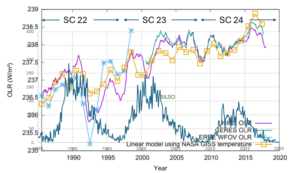
Figure 2. Plot of HIRS (purple line, the high-resolution Infrared Radiation Sounder on NOAA and EUMETSAT’s satellites), CERES (green line, Clouds and Earth’s Radiant Energy System instruments), and ERBE (light blue line, Earth Radiation Budget Satellite) OLR at the top of the atmosphere. GISS global average surface temperature is shown in yellow. The solar cycles (SC) during this period are noted as well as the SILSO sunspot count in dark green. After (Dewitte & Clerbaux, 2018).
Figure 2 suggests that Held and Soden’s model of how the greenhouse effect works is incorrect or CO2 is not the reason for the recent warming, as explained by Javier Vinós here. Notice the qualitative pattern in OLR matches each solar cycle in shape. This suggests that the solar cycles contribute to the OLR pattern. So, while the increase in CO2 might influence recent warming, the variations throughout a solar cycle also likely contribute.
ENSO and the AMO
From 1950-1975 Dewitte’s cumulative MEI (the Multivariate ENSO Index) was decreasing, suggesting a period of strong Las Niñas. From 1975 to 1998 it was increasing, suggesting a period strong Los Niños. From 1998-2014 it was flat and Los Niños and Las Niñas were more or less equal. This is illustrated in figure 3.
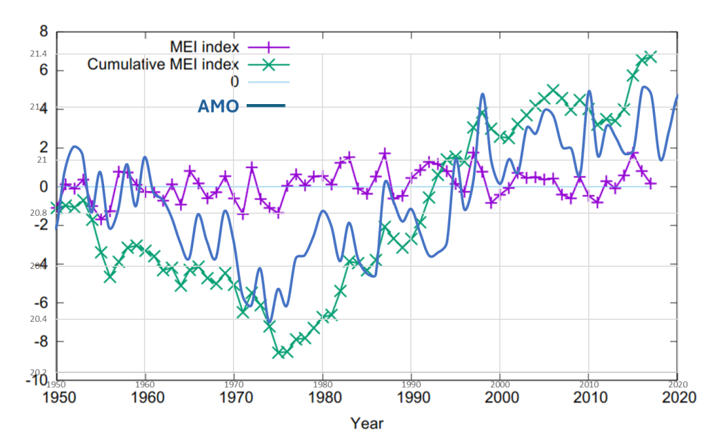
Figure 3. Cumulative MEI Index, MEI, and AMO. After: (Dewitte & Clerbaux, 2018).
The deep blue line in figure 3, with no marks, is the AMO or Atlantic Multidecadal Oscillation. Notice that it roughly corresponds with the cumulative MEI index. This suggests that the North Atlantic sea surface temperatures are related to the frequency of Los Niños and Las Niñas in some fashion (An, Wu, Zhou, & Liu, 2021), or they both follow some other influence, like solar variability. Again, it looks less likely that CO2 is the “climate control knob” (IPCC, 2021, p. 179).
Clouds and ECS
From (Loeb, et al., 2021):
“Climate is determined by how much of the sun’s energy the Earth absorbs and how much energy Earth sheds through emission of thermal infrared radiation. Their sum determines whether Earth heats up or cools down.”
This is a vast oversimplification, as it ignores the impact of energy residence time which varies continuously. Energy residence time varies as a function of atmospheric and oceanic circulation trends, which are influenced by solar variability (see figures 5.3, 5.4, and 5.5 here).
Loeb, 2021 notes that an increase in absorbed energy by the Earth from 2005 to 2019 is accompanied by a decrease in cloud cover (see figure 4). The decrease in cloud cover reduces reflection of incoming solar energy, but also decreases absorption of outgoing surface IR by clouds. Dewitte (see above) reports an increase in outgoing longwave radiation at the same time.
Kauppinen & Malmi, 2019 report that low cloud cover has decreased, as shown in their figure 2.
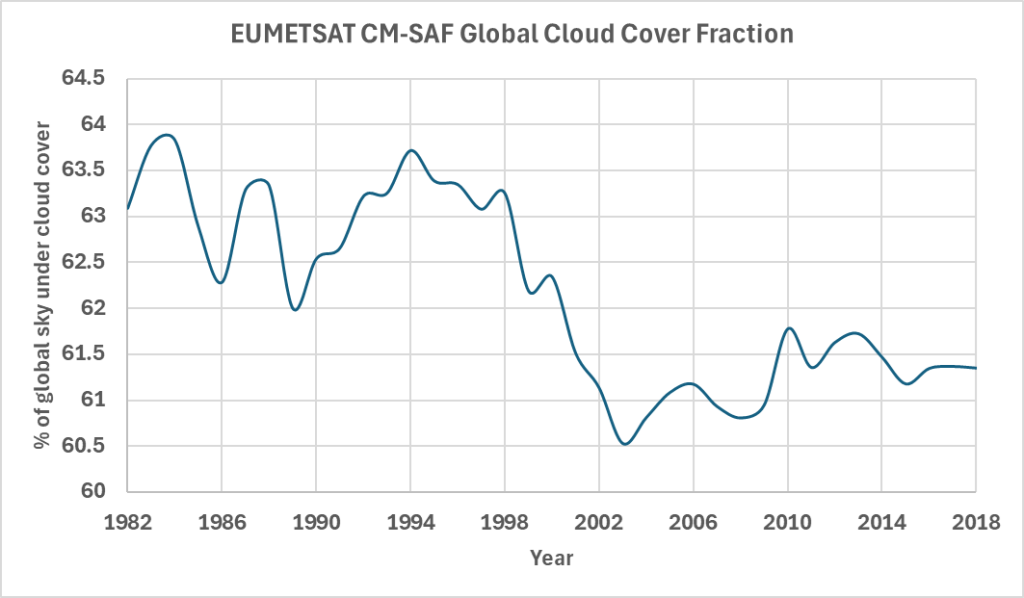
Figure 4. Total global cloud cover as a percent of the sky. Data from EUMETSAT CM-SAF.
As explained in Kauppinen & Malmi, 2019 low cloud cover (as well as total cloud cover) decreases as the “pause” in global warming starts around the year 2000. Overall, as low cloud cover increases 1%, global average surface temperature decreases 0.11°C on average. As a function of EUMETSAT global cloud fraction, the HadCRUT4 global surface temperature decreases 0.15°C per one percent total cloud cover, as illustrated in figure 5.
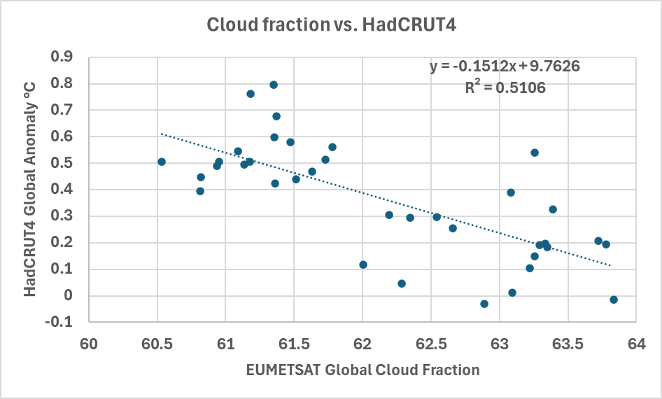
Figure 5. EUMETSAT global cloud cover versus HadCRUT4 global average surface temperature. Data from the UK Met Office and EUMETSAT CM-SAF.
The data displayed in figures 2 through 5 cannot be explained as a function of the monotonically increasing atmospheric CO2 and other greenhouse gases and their so-called “heat trapping” or “OLR delaying” capabilities. While additional greenhouse gases may have some influence on increasing surface temperatures, we cannot see any sign of this influence in these data.
Ceppi & Nowack, 2021 try to show that cloud cover responds to surface temperature and figure 5 appears to support that idea. However, they and the IPCC believe that changes in cloud cover due to a warming surface increase warming on net, that is cloud cover changes due to surface warming are a net positive feedback (IPCC, 2021, p. 95). They are vague in their language and do not claim that increasing cloud cover increases warming, rather they say the net change in cloud cover due to surface warming is a positive feedback. Thus, they break clouds up into types, some are net warming, and some are net cooling, with the overall change being positive.
Figures 4 and 5, and the work of Kauppinen & Malmi suggest that an increase in clouds, as the world warms, decreases warming. Figure 2 suggests that OLR increases as the world warms and cloud cover decreases, this is not what one would expect if cloud cover changes are a net positive feedback to surface warming. However, the two ideas are not necessarily incompatible as neither the IPCC, nor Ceppi & Nowack say increasing cloud cover increases warming, they say “cloud cover changes” increase warming on net. Time will tell if their complex hypothesis is correct.
Ceppi & Nowack explicitly assume that greenhouse gases are causing global warming according to the RCP4.5 scenario. They do not consider the possibility that variations in solar activity (figure 2) or ocean oscillations (like the AMO plotted in figure 3) have an impact. Loeb, 2021 does discuss changes in the PDO, but not as a driver in climate change, just a type of internal natural variability.
As Ceppi & Nowak report, ECS correlates very well with cloud cover, see figure 2 here. It is also true that cloud cover is the most uncertain feedback in greenhouse gas climate models and climate modelers have reported fiddling with their cloud parameters (Koonin, 2021, p. 93) to achieve a pre-determined ECS. It lessens our confidence in climate models when the most uncertain and poorly understood component of them (clouds) is used to create a desired result. Further, as AR6 WGI reports on page 927, the ECS calculated by climate models is becoming more uncertain and the reason given is that the modelers are fiddling more with their cloud parameters to try and match cloud observations. Something is clearly amiss in modern climate models, and the problem is getting worse with time.
EEI (Earth Energy Imbalance)
The net radiation in or out is the Earth Energy Imbalance or EEI. When it is positive the Earth is warming and collecting heat and when it is negative the Earth is cooling. Because most solar energy absorbed on Earth’s surface is stored in the oceans (~90%) the ocean heat content is a sensitive indicator of long-term EEI and can be used as a check and calibration point for satellite radiation measurements which are not accurate enough on their own to directly measure EEI (Loeb, et al., 2022).
Table 1 in (Loeb, et al., 2022) lists the absorbed solar radiation (ASR), the outgoing longwave radiation (OLR), and the net radiation in (positive) and out (negative) for various satellite instrument analyses. The trends vary from 0.026 to 0.42 W/m2/decade ±~.24. This is a fairly large and uncertain difference. The numbers are positive since the world is warming.
The actual EEI and the trend in the EEI are unknown, but ocean heat content estimates from 2005 to 2019 suggest it is small and between 0.24 and 0.98 (±~0.7) W/m2/decade according to Table 4 in (Loeb, et al., 2022). ARGO has greatly increased our knowledge of ocean temperature to a depth of 2,000 meters, but trends in temperature below 2,000 meters and under sea ice are still largely unknown. It seems safe to conclude that the trend, since 2000, is somewhere between ~-0.7 and ~1.5 W/m2/decade and more likely positive than negative, because the Earth is warming, but beyond that it is hard to say. The total incoming solar radiation and the total outgoing longwave radiation are large numbers, with large uncertainty, and the difference between the two is very small and below the accuracy of current measurements.
The change in ocean heat content is useful as a check, but we don’t have a good handle on ocean temperatures, either aerially or at depth. ARGO improves things, but the coverage is still poor. As for measuring incoming and outgoing radiation, there are problems in the eastern Pacific, the Arctic, and in many other areas. For a complete discussion of the problems estimating the EEI trend the interested reader is referred to (Loeb, et al., 2022).
Conclusions
As I’ve written before the current group of IPCC/CMIP climate models do not compare well with observations, and unfortunately, in the tropics they do better if the man-made portion of the enhanced greenhouse effect is removed. It seems that the conceptual model they have pursued since 1990 (the first IPCC report) that CO2 is the “control knob” for global warming is flawed. There is abundant evidence that climate has many drivers, and man-made CO2 is only one, and one that may not be that significant. It is way past time that the IPCC quit pushing this man-made climate change idea and go back to the drawing board and develop a new conceptual model that makes sense with the data presented in this post.
Download the bibliography here.
