By Andy May
You can read this post in German here, courtesy of Christian Freuer.
Here we go again, writing on the proper use of statistics in climate science. Traditionally, the most serious errors in statistical analysis are made in the social sciences, with medical papers coming in a close second. Climate science is biting at their heels.
In this case we are dealing with a dispute between Nicola Scafetta, a Professor of Atmospheric Physics at the University of Naples and Gavin Schmidt, a blogger at RealClimate.org, a climate modeler, and director at NASA’s Goddard Institute for Space Studies (GISS).
Scafetta’s original 2022 paper in Geophysical Research Letters is the origin of the dispute (downloading a pdf is free). The essence of the paper is that CMIP6 global climate models (GCMs) that produce an ECS (Equilibrium Climate Sensitivity) higher than 3°C/2xCO2 (“°C/2xCO2” means °C per doubling of CO2) are statistically significantly different (they run too hot) from observations since 1980. This result is not surprising and is in line with the recent findings by McKitrick and Christy (2020). The fact that the AR6/CMIP6 climate models run too hot and that it appears to be a function of too-high ECS is acknowledged in AR6:
“The AR5 assessed with low confidence that most, though not all, CMIP3 and CMIP5 models overestimated the observed warming trend in the tropical troposphere during the satellite period 1979-2012, and that a third to a half of this difference was due to an overestimate of the SST [sea surface temperature] trend during this period. Since the AR5, additional studies based on CMIP5 and CMIP6 models show that this warming bias in tropospheric temperatures remains.”
(AR6, p. 443)
And:
“Several studies using CMIP6 models suggest that differences in climate sensitivity may be an important factor contributing to the discrepancy between the simulated and observed tropospheric temperature trends (McKitrick and Christy, 2020; Po-Chedley et al., 2021)”
(AR6, p. 443)
The AR6 authors tried to soften the admission with clever wording, but McKitrick and Christy showed that the AR5/CMIP5 models are too warm in the tropical troposphere and fail to match observations at a statistically significant level. Yet, regardless of the evidence that AR5 was already too hot, AR6 is hotter, as admitted in AR6 on page 321:
“The AR5 assessed estimate for historical warming between 1850–1900 and 1986–2005 is 0.61 [0.55 to 0.67] °C. The equivalent in AR6 is 0.69 [0.54 to 0.79] °C, and the 0.08 [-0.01 to 0.12] °C difference is an estimate of the contribution of changes in observational understanding alone (Cross-Chapter Box 2.3, Table 1).”
(AR6, p. 321).
So, we see that the AR6 assessment that the AR6 and AR5 climate sensitivity to CO2 may be too high and that AR6 is worse than AR5 supports the work that Scafetta, McKitrick, and Christy have done in recent years.
Now let’s look at the dispute on how to compute the statistical error of the mean warming from 1980-1990 to 2011-2021 between Scafetta and Schmidt. Schmidt (2022)’s objections to Scafetta’s error analysis are posted on his blog here. Scafetta’s original Geophysical Research Letters paper was later followed by a more extended paper in Climate Dynamics (Scafetta N., 2022b) where the issue is discussed in detail in the first and second appendix.
Scafetta (2022a)’s analysis of climate model ECS
The essence of Scafetta’s argument is illustrated in figure 1.

Figure 1. Plots of climate model results are shown in red and ECMWF ERA5 weather reanalysis observations are shown in blue. The top two plots show model runs that result in ECS calculations greater than 3°C/2xCO2 and the lower plot those with ECS less than 3°C/2xCO2. Plot from (Scafetta N., 2022a)
In figure 1 we see that when ECS is greater than 3°C/2xCO2 the models run hot. The righthand plots show a comparison of the mean difference between the observations and models between the 11-year periods of 1980-1990 and 2011-2021. Scafetta’s 2022a full analysis is contained in his Table 1 where 107 CMIP6 GCM average simulations for the historical + SSP2-4.5, SSP3-7.0, and SSP5-8.5 IPCC greenhouse emissions scenarios provided by Climate Explorer are analyzed. The ERA5-T2m[1] mean global surface warming from 1980-1990 to 2011-2021 was estimated to be 0.578°C from the ERA5 worldwide grid. The IPCC/CMIP6 climate model mean warming is significantly higher for all the models plotted when ECS is greater than 3°C/2xCO2.
Schmidt’s analysis
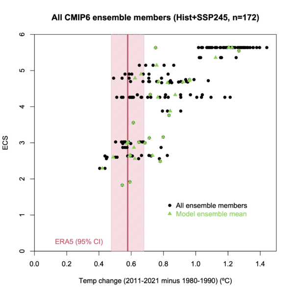
The plots shown on the right in figure 1 are the essence of the debate between Scafetta and Schmidt. The data plotted by Schmidt (shown in our figure 2) is slightly different but shows the same thing.

Figure 2. Schmidt’s plot of IPCC/CMIP6 modeled ECS versus ERA5 reanalysis observations. The green dots are the model ensemble means used in Scafetta’s plot (figure 1) and the black dots are individual model runs. The pink band is Schmidt’s calculation of the ERA5 observational uncertainty
In figure 2 we see that the only model ECS ensemble mean estimates (green dots) that equal or fall around the ERA5 weather reanalysis mean difference between 1980-1990 and 2011-2021 are ECS estimates of 3°C/2xCO2 or less. All ensemble ECS estimates above 3°C/2xCO2 run too hot. Thus, on the basic data Schmidt agrees with Scafetta, which is helpful.
The Dispute
The essence of the dispute is how to compute the 95% uncertainty (the error estimate) of the 2011-2021 ERA5 weather reanalysis mean relative to the 1980-1990 period. This error estimate is used to decide whether a particular model result is within the margin of error of the observations (ERA5) or not. Scafetta computes a very small ERA5 error range of 0.01°C (Scafetta N. , 2022b, Appendix) from similar products (HadCRUT5, for example) because ECMWF (European Centre for Medium-Range Weather) provides no uncertainty estimate with their weather reanalysis product (ERA5), so it must be estimated. Schmidt computes a very large ERA5 margin of error of 0.1°C using the ERA5 standard deviation for the period. It is shown with the pink band in figure 2. This is the critical value in deciding which differences between the climate model results and the observations are statistically significant.
If we assume that Scafetta’s estimate correct, figures 1 and 2 show that all climate model simulations (the green dots in figure 2) for the 21 climate models with ECS >3°C and the great majority of their simulation members (the black dots) are obviously too warm at a statistically significant level. Whereas, assuming Schmidt’s estimate correct, figure 2 suggests that three climate models with ECS>3°C partially fall within the ERA5 margin of error while the other 18 climate models run too hot.
Although Schmidt’s result does not appear to significantly change the conclusion of Scafetta (2022a, 2022b) that only the climate models with ECS<3.01°C appear to best hindcast the warming from 1980-1990 to 2011-2021, it is important to discuss the error issue. I will refer to the standard stochastic methods for the evaluation of the error of the mean discussed in the classical textbook on error analysis by Taylor (1997).
In the following I repeat the calculation made by Schmidt and comment on them using the HadCRUT5.0.1.0 annual mean global surface temperature record instead of the ERA5-T2m because it is easier to get, it is nearly equivalent to ERA5-T2m, and especially because it also reports the relative stochastic uncertainties for each year, which, as already explained, is a crucial component to evaluating the statistical significance of any differences between reality and the climate models.
Schmidt’s estimate of the error of the mean (the pink bar in Figure 2) is ± 0.1°C (95% confidence). He obtained this value by assuming that the interannual variability in the ERA5-T2m from 2011 to 2021 from the decadal mean is random noise. Practically, he calculated the average warming (0.58°C) from 2011 to 2021 using the ERA5-T2m temperature anomalies relative to the 1980-1990 mean. That is, he “baselined” the values to the 1980-1990 mean. Then he estimated the error of the mean by computing the standard deviation of the baselined values from 2011 to 2021, he then divided this standard deviation by the root of 11 (because there are N=11 years) and, finally, he multiplied the result by 1.96 to get the 95% confidence. Download a spreadsheet performing Schmidt’s and Scafetta’s calculations here.
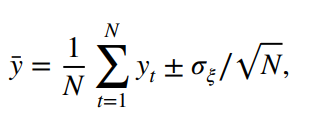
Figure 3 shows Schmidt’s equation for the error of the mean. When this value is multiplied by 1.96, to get the 95% confidence, it gives an error of ± 0.1°C.

Figure 3. The equation Schmidt used to compute the error of the mean for the ERA5 data
The equations used by Schmidt are those reported in Taylor (1997, pages 100-102). The main concern with Schmidt’s approach is that Taylor clearly explains that the equation in figure 3 for the error of the mean only works if the N yearly temperature values (Ti) are random “measurements of the same quantity x.” For example, Taylor (page 102-103) uses the above equation to estimate the error of the mean for the elastic constant k of “one” spring by using repeated measurements with the same instrument. Since the true elastic constant is only one value, the variability of the repeated measurements can be interpreted as random noise around a mean value whose standard deviation is the Standard Deviation of the Mean (SDOM).
In using the SDOM, Schmidt et al. implicitly assume that each annual mean temperature datum is a measurement of a single true decadal value and that the statistical error for each datum is given by its deviation from that decadal mean. In effect, they assume that the “true” global surface temperature does not vary between 1980 and 1990 or 2011-2021 and all deviations from the mean (or true) value are random variability.
However, the interannual variability of the global surface temperature record over these two decades is not random noise around a decadal mean. The N yearly mean temperature measurements from 2011 to 2021 are not independent “measurements of the same quantity x” but each year is a different physical state of the climate system. This is easily seen in the plot of both decades in this spreadsheet. The x-axis is labeled 2010-2022, but for the orange line, it is actually 1979-1991, I did it this way to show the differences in the two decades. Thus, according to Taylor (1997), SDOM is not the correct equation to be adopted in this specific case.
As Scafetta (2022b) explains, the global surface temperature record is highly autocorrelated because it contains the dynamical interannual evolution of the climate system produced by ENSO oscillations and other natural phenomena. These oscillations and trends are a physical signal, not noise. Scafetta (2022b) explains that given a generic time series (yt) affected by Gaussian (randomly) distributed uncertainties ξ with standard deviation σξ, the mean and the error of the mean are given by the equation in figure 4.

Figure 4. The proper equation for computing the uncertainty in the mean of global surface temperature over a period in which the mean is changing
The equation in figure 4 gives an error of 0.01°C (at the 95% confidence level, see the spreadsheet here for the computational details). If the standard deviation of the errors are not strictly constant for each datum, the standard error to be used in the above equation is the square root of the mean of the squared uncertainties for each datum.
Scafetta’s equation derives directly from the general formula for the error propagation discussed by (Taylor, 1997, p. 60 and 75). Taylor explains that the equations on pages 60 and 75 must be adopted for estimating the error of a function of “several” independent variables each affected with an individual stochastic error, corresponding to different physical states, such as the average of a global surface temperature record of N “different” years. The uncertainty of the function (e.g., the mean on N different quantities) only depends on the statistical error of each quantity, not on the variability of the various quantities from their mean.
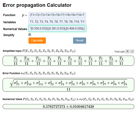
We can use an error propagation calculator tool available on the internet to check our calculations. I uploaded the annual mean ERA5 temperature data and the respective HadCRUT5 uncertainties and had the calculator evaluate the mean with its relative error. The result is shown in Figure 5.

Figure 5. The proper equation for computing the uncertainty in the mean of global surface temperature over a period of N=11 different years characterized by different yearly temperatures means
Schmidt’s calculation of the standard deviation of the mean (SDOM) is based on the erroneous premise that he is making multiple measurements of the same thing, using the same method, and that, therefore, the interannual variability from the decadal mean is some kind of random noise that can be considered stochastic uncertainty. None of these conditions are true in this case. The global yearly average surface temperature anomaly is always changing for natural reasons, although its annual estimates are also affected by a small stochastic error such as those incorporated into Scafetta’s calculation. According to Taylor, it is only the errors of measure of the yearly temperature means that can determine the error of the 11-year mean from 2011 to 2021.
As Scafetta writes in the appendix to Scafetta 2022b, HadCRUT5’s global surface temperature record includes its 95% confidence interval estimate and, from 2011 to 2021, the uncertainties for the monthly and annual averages are monthly ≈ 0.05°C and annual ≈ 0.03°C. Berkeley Earth land/ocean temperature record uncertainty estimates are 0.042°C (monthly), 0.028°C (annual), and 0.022°C (decadal). The longer the time period, the lower the error of the mean becomes.
Each of the above values, year-by-year, must averaged and divided by the square-root of the number of years (in this case 11) to determine the error of the mean. In our case, the HadCRUT5 error of the mean for 2011-2021 is 0.01°C. Scafetta’s method allows for the “true” value to vary in each year, Schmidt’s method does not.
The observations used for the ERA5 weather reanalysis are very nearly the same as those used in the HadCRUT5 dataset (Lenssen et al., 2019; Morice et al., 2021; Rohde et al., 2020). As Morice et al. note, the MET Office Hadley Centre uses ERA5 for quality control.
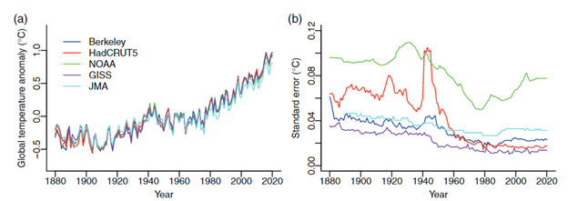
Lenssen et al., which includes Gavin Schmidt as a co-author, does an extensive review of uncertainty in several global average temperature datasets, including ERA5. Craigmile and Guttorp provide the plot in figure 6 of the estimated yearly standard error in several global surface temperature records: GISTEMP, HadCRUT5, NOAA, GISS, JMA and Berkeley Earth.

Figure 6. Total uncertainty for three global temperature anomaly datasets. These datasets should have a similar uncertainty as ERA5. Source: (Craigmile & Guttorp, 2022)
Figure 6 shows that from 1980 to 2021, at the annual scale and at 95% confidence, the standard error of the uncertainties is much less than Schmidt’s error of the mean of 0.10°C, which, furthermore, is calculated on a time scale of 11 years. The uncertainties reported in Figure 6 are not given by the interannual temperature variability around a decadal mean. This result clearly indicates that Schmidt’s calculation is erroneous because at the 11-year time scale the error of the mean must be significantly smaller (by the root of 11 = 3.3) than the annual value.
Scafetta (2022b) argues that the errors for the annual mean of the ERA5-T2m should be of the same order of magnitude as those of other temperature reconstructions, like the closely related HadCRUT5 dataset. Thus, the error at the decadal scale must be negligible, about ±0.01°C, and this result is also confirmed by the online calculator tools for estimating the error of given functions of independent variables as shown in figure 5.
The differences between Scafetta and Schmidt are caused by the different estimates of ERA5 error. I find Scafetta’s much more realistic.
Patrick Frank helped me with this post, but any errors are mine alone.
Download the bibliography here.
