In my last post, it was suggested that Michael Mann’s 2008 reconstruction (Mann, et al., 2008) was similar to Moberg’s 2005 (Moberg, Sonechkin, Holmgren, Datsenko, & Karlen, 2005) and Christiansen’s 2011/2012 reconstructions. The claim was made by a commenter who calls himself “nyolci.” He presents a quote, in this comment, from Christiansen’s co-author: Fredrik Charpentier Ljungqvist:
“Our temperature reconstruction agrees well with the reconstructions by Moberg et al. (2005) and Mann et al. (2008) with regard to the amplitude of the variability as well as the timing of warm and cold periods, except for the period c. AD 300–800, despite significant differences in both data coverage and methodology.” (Ljungqvist, 2010).
A quick google search uncovers this quote in a paper by Ljungqvist in 2010 (Ljungqvist, 2010), one year before the critical reconstruction by Christiansen and Ljungqvist in 2011 (Christiansen & Ljungqvist, 2011) and two years before their 2012 paper (Christiansen & Ljungqvist, 2012). It turns out that Ljungqvist’s 2010 reconstruction is quite different than those he did with Christiansen over the next two years. All the reconstructions are of the Northern Hemisphere. Ljungqvist’s and Christiansen’s are of the extra-tropical (> 30°N) Northern Hemisphere and Moberg’s and Mann’s are supposed to be of the whole Northern Hemisphere, but the big differences lie in the methods used.
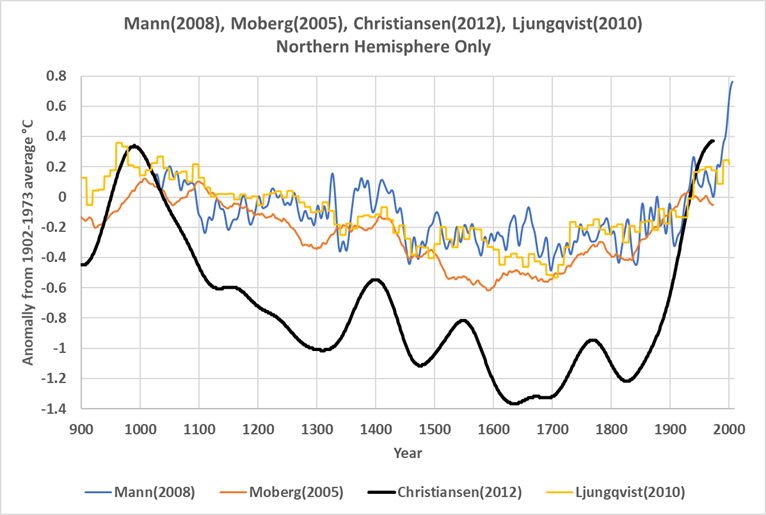
With regard to the area covered, Moberg only has one proxy south of 30°N. Mann uses more proxies, but very few of his Northern Hemisphere proxies are south of 30°N. Figure 1 shows all the reconstructions as anomalies from the 1902-1973 average.

Figure 1. A comparison of all four reconstructions. All are smoothed with 50 year moving averages except for the Ljungqvist (2010) reconstruction which is a decadal record. All have been shifted to a common baseline (1902-1973) to make them easier to compare. Ljungqvist(2010) is a decadal record.
As Figure 1 shows, the original Ljungqvist(2010) record is similar to Mann(2008) and Moberg(2005). A couple of years after publishing Ljungqvist(2010), Ljungqvist collaborated with Bo Christiansen and made the record labeled Christiansen(2012). It starts with the same proxies as Ljungqvist(2010), but uses a different method of combining the proxies into a temperature record that they call “LOC.”
In 2008, Michael Mann created several different proxy records, the one plotted in Figure 1 is the Northern Hemisphere EIV Land and Ocean record. EIV stands for “error-in-variables” and is a total least squares regression methodology. Mann states at the beginning of his paper that he would address the criticism (“suggestions”) in the 2006 National Research Council report (National Research Council, 2006). The result is a complex and hard to follow discussion of various statistical techniques used on various combinations of proxies. He doesn’t have one result, but many, then he compares them to one another.
Moberg (2005) also uses regression to combine his proxies but characterizes them by resolution to preserve more short-term variability. The statistical technique used by Ljungqvist in his 2010 paper is similar and called “composite-plus-scale” or CPS. This technique is also discussed by Mann in his 2008 paper and he found that it produced similar results to his EIV technique. Since these three records were created using similar methods, they all agree quite well.
Christiansen and Ljungqvist (2011 and 2012)
Everyone admits that using regression-type methods to combine multiple proxies into one temperature reconstruction reduces and dampens the temporal resolution of the resulting record. Instrumental (thermometer) measurements are normally accurately dated, at least down to a day or two. Proxy dates are much less accurate, many of them are not even known to the year. Those that are accurate to a year often only reflect the temperature during the growing season, during winter or during the flood season. Ljungqvist’s 2010 record is only decadal due to these problems.
Inaccurate dates, no matter how carefully they are handled, lead to mismatches when combining proxy records and result in unintentional smoothing and dampening of high-frequency variability. The regression process itself, leads to low-frequency variability, Christiansen and Ljungqvist write:
“[Their] reconstruction is performed with a novel method designed to avoid the underestimation of low-frequency variability that has been a general problem for regression-based reconstruction methods.”
Christiansen and Ljungqvist devote a lot of their paper to explaining how regression-based proxy reconstructions, like the three shown in Figure 1, underestimate low-frequency variability by 20% to 50%. They list many papers that discuss this problem. These reconstructions cannot be used to compare current warming to the pre-industrial era. The century-scale detail, prior to 1850, simply isn’t there after regression is used. Regression reduces statistical error, but at the expense of blurring critical details. Therefore Mann adding instrumental temperatures onto his record in Figure 1 makes no sense. You might as well splice a satellite photo onto a six-year-old child’s hand-drawn map of a town.
Christiansen and Ljungqvist make sure all their proxies have a good correlation to the local instrumental temperatures. About half their proxies have annual samples and half decadal. The proxies that correlate well with local (to the proxy) temperatures are then regressed against the local instrumental temperature record. That is the local temperature is the independent variable or the “measurements.” The next step is to simply average the local reconstructed temperatures to get the extratropical Northern Hemisphere mean. Thus, only minimal and necessary regression is used, so as not to blur the resulting reconstruction.
Discussion
Regression does reduce the statistical error in the predicted variable, but it reduces variability significantly, up to 50%. So, using regression to build a proxy temperature record to “prove” recent instrumental measured warming is anomalous is disingenuous. The smoothed regression-based records in Figure 1 show Medieval Warm Period (MWP) to Little Ice Age (LIA) cooling of about 0.8°C, this is more likely to be 1°C to 1.6°C, or more, after correcting for the smoothing due to regression. There is additional high-frequency smoothing, or dampening, of the reconstruction due to poorly dated proxies.
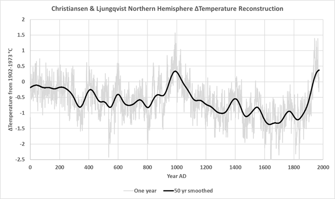
The more cleverly constructed Christiansen and Ljungqvist record (smoothed) shows a 1.7°C change, which is more in line with historical records, borehole temperature data, and glacial advance and retreat data. See Soon and colleagues 2005 paper for a discussion of the evidence (Soon, Baliunas, Idso, Idso, & Legates, 2003b). Christiansen and Ljungqvist stay much closer to the data in their analysis to avoid distorting it, this makes it easier to interpret. Figure 2 shows the same Christiansen and Ljungqvist 2012 curve shown in black in Figure 1 and the yearly Northern Hemisphere averages.

Figure 2. Christiansen and Ljungqvist 2012 50-year smoothed reconstruction and the one-year reconstruction. The black line is the same as in Figure 1, but the scale is different.
The one-year reconstruction is the fine gray line in Figure 2. It is a simple average of Northern Hemisphere values and is unaffected by regression, thus it is as close to the data as possible. Maximum variability is retained. Notice how fast temperatures vary from year-to-year, sometimes by over two degrees in just one year, 542AD is an example. From 976AD to 990AD temperatures rose 1.6°C. These are proxies and not precisely dated, so they are not exact values and take them with a grain of salt, but they do show us what the data say, because they are minimally processed averages.
The full range of yearly average temperatures over the 2,000 years shown is 4.5°C. The full range of values with the 50-year smoothing is 1.7°C. Given that nearly half of the proxies used are decadal, and linearly interpolated to one-year, I trust the 50-year smoothed record more than the yearly record over the long-term. But, seeing the variability in the one-year record is illuminating, it reinforces the foolishness of comparing modern yearly data to ancient proxies. Modern statistical methods and computers are useful, but sometimes they take us too far away from the data and lead to misinterpretations. I think that often happens with paleo-temperature reconstructions. Perhaps with modern temperature records as well.
It is quite possible that we will never know if past climatic warming events were faster than the current warming rate or not. The high-quality data needed doesn’t exist. What we do know for sure, is that regression methods, all regression methods, significantly reduce low-frequency variability. Mixing proxies with varying resolutions and imprecise dates, using regression, destroys high-frequency variability. Comparing a proxy record to the modern instrumental record tells us nothing. Figure 1 shows how important the statistical methods used are, they are the key difference in those records. They all have access to the same data.
Download the bibliography here.

Andy May, now retired, was a petrophysicist for 42 years. He has worked on oil, gas and CO2 fields in the USA, Argentina, Brazil, Indonesia, Thailand, China, UK North Sea, Canada, Mexico, Venezuela and Russia. He specializes in fractured reservoirs, wireline and core image interpretation and capillary pressure analysis, besides conventional log analysis. He is proficient in Terrastation, Geolog and Powerlog software. His full resume can be found on linkedin or here: AndyMay
