Reposted from Andy May Petrophysicist
Many viewers of Climate: The Movie have asked for more information on the topics discussed. In response, I selected the following 70 key statements from the movie and provide references and context for the statements here. Sometimes the statements are slightly paraphrased from what was said for brevity. The statements are listed in the same order as they appear in the movie. The references, illustrations, and links below are my attempt to clarify the statements, provide context, and support the idea behind the phrase or sentence.
I received help from Dr. Willie Soon and Marty Cornell in building this bibliography. My thanks to both.
Trillions of dollars at stake.
World Economic Forum and McKinsey Report.
The Swiss Re Group reports US$270 trillion is needed meet 2050 net-zero targets.
There is no evidence of a Climate Emergency.
These “27 estimates are a thin basis for drawing definitive conclusions about the total welfare impacts of climate change. Moreover, the 11 estimates for warming of 2.5 C indicate that researchers disagree on the sign of the net impact: 3 estimates are positive and 8 are negative. Thus it is unclear whether climate change will lead to a net welfare gain or loss.”
Tol, 2018
Lomborg, B. (2020, July). Welfare in the 21st century: Increasing development, reducing inequality, the impact of climate change, and the cost of climate policies,. Technological Forecasting and Social Change, 156. doi:10.1016/j.techfore.2020.119981
Tol, R. (2023). Costs and benefits of the Paris Climate Targets. Climate Change Economics, 14(4). doi:10.1142/S2010007823400031
Tol, R. S. (2018). The Economic Impacts of Climate Change. Review of Environmental Economics and Policy, 12(1), 4-25. doi:10.1093/reep/rex027
Skepticism is career suicide and might be criminalized.
Wielicki and Robert Kennedy Jr.
Deniers are evil and should be shunned.
No such thing as “Settled Science.”
Unsettled, What Climate Science tells us, what it doesn’t, and why it matters, by Steven Koonin.
Climate proxies
A good overview of climate proxies:
Patalano, R., & Roberts, P. (2021). Climate proxies. In D. T. Potts, & E. Harkness, The Encyclopedia of Ancient History. John Wiley & Sons. doi:10.1002/9781119399919.eahaa00609
For a discussion of many of the best global temperature proxies that cover the past 12,000 years see Climate Catastrophe! Science or Science Fiction?, 2018, pp. 95-107.
May, A. (2018). Climate Catastrophe! Science or Science Fiction? American Freedom Publications LLC.
Temperature for the past 500 million years
Scotese, C., Song, H., Mills, B. J., & Meer, D. v. (2021, January ). Invited Review: Phanerozoic Paleotemperatures: The Earth’s Changing Climate during the Last 540 Million Years. Earth-Science Reviews.
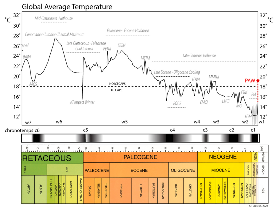
Figure 1. Scotese’s reconstruction of the past 125 million years. Major climatic changes are identified, as well as the IPCC projected anthropogenic global warming (PAW). (Scotese, Song, Mills, & Meer, 2021). Notice the PAW has recently (geologically speaking) been exceeded, it is not unusual.
When was the Earth as cold as now?
As can be seen in figure 2, temperatures have not been as cold as today for over 250 million years. Figure 2 is by the Smithsonian and from NOAA’s climate.gov website.
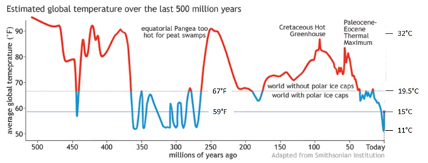
Figure 2. A reconstruction of Phanerozoic (past 540 million years) temperatures by Scott Wing, Brian Huber, and Chris Scotese at the Smithsonian.
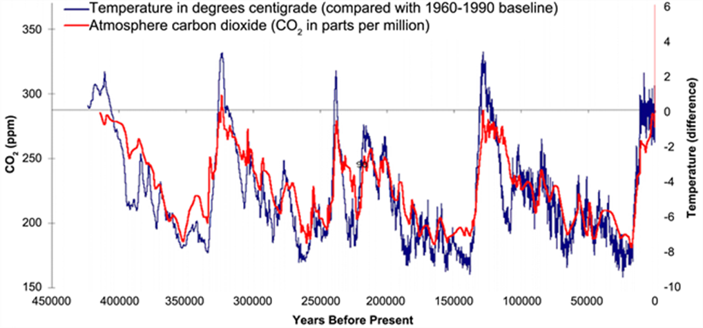
Figure 3. The most recent 420,000 years of the 2.5 million year Late Cenozoic Ice Age as seen in Antarctic ice core data collected by Petit, et al, 1999. The CO2 is in parts per million atmospheric concentration and the temperatures are anomalies from the present. Plot from Watts and Pacnik, 2012.
The Late Cenozoic Ice Age (the past 2.6 million years) is characterized by a series of glacial advances (colder periods) and glacial retreats (warmer periods) that are about 100,000 years apart. We are currently in a period of glacial retreat, also called an “interglacial.” Our interglacial is named the “Holocene” and is the most recent 12,000 years. Notice the changes in CO2 (in red) tend to follow the changes the temperature (in blue), suggesting that CO2 did not cause the temperature change.
Also see: David Legates and Euan Mearns.
Holocene warm period or the “Holocene Climatic Optimum.”
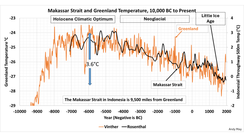
Figure 4. The Holocene, with its major periods identified.
The two temperature proxies shown are from the Indonesian Makassar Strait and from Greenland. While the Makassar Strait is technically in the Southern Hemisphere, the 500-meter water there flows from the Northern Hemisphere and represents sea-surface temperatures in the North Pacific. Thus, the proxies represent the Northern Hemisphere, but they are 9,500 miles apart. The Northern Hemisphere is where the largest temperature changes occur. The Holocene Climatic Optimum is about 3.6°C warmer at these two locations than the Little Ice Age, also known as the “pre-industrial.” The source of the figure and more explanation is here.
There has been an attempt to claim that the Holocene Climatic Optimum was actually colder than today by Bova, et al. (2021), but the paper has drawn two serious criticisms (see Laepple, et al., 2022 and Zhang & Chen, 2021) and undergone a major revision.
Bova, S., Rosenthal, Y., & Liu, Z. (2021). Seasonal origin of the thermal maxima at the Holocene and the last interglacial. Nature, 589, 548-553. doi:10.1038/s41586-020-03155-x
Laepple, T., Shakun, J., He, F., & Marcott, S. (2022). Concerns of assuming linearity in the reconstruction of thermal maxima. Nature, 607. doi:10.1038/s41586-022-04831-w
Zhang, X., & Chen, F. (2021). Non-trivial role of internal climate feedback on interglacial temperature evolution. Nature, 600. doi:10.1038/s41586-021-03930-4
Holocene Climatic Optimum and the beginning of civilization
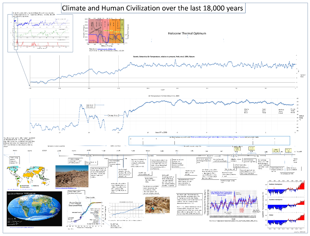
Figure 5. An overview of the development of human civilization over the past 18,000 years and its relationship to major climate changes. To download the full resolution version click here. Major events in the development of human civilization are noted, both Greenland and Antarctic ice core temperatures are plotted. Source.
Little Ice Age/pre-industrial
Behringer, W. (2010). A Cultural History of Climate. Cambridge, UK: Polity Press
Also see these interesting articles on the Little Ice Age/pre-industrial by Paul Homewood, Geoffrey Parker, and Soon et al.
Soon, W., Baliunas, S., Idso, C., Idso, S., & Legates, D. (2003b). Reconstructing Climatic and Environmental Changes of the Past 1000 years: A Reappraisal. Energy and Environment, 14(2&3).
Roman Warm Period
A brief overview of the evidence for the Roman Warm Period in Europe, with a bibliography, can be seen at CO2science.org here. More information and references are given here. The topic is also covered by Soon, et al.:
Soon, W., Baliunas, S., Idso, C., Idso, S., & Legates, D. (2003b). Reconstructing Climatic and Environmental Changes of the Past 1000 years: A Reappraisal. Energy and Environment, 14(2&3). Retrieved from https://journals.sagepub.com/doi/abs/10.1260/095830503765184619
Central England Temperature Record
The Central England Temperature record is now maintained by the Hadley Centre. It can be viewed and downloaded here. A discussion of the climatic significance of the record is given in Baliunas, et al.
Baliunas, S., Frick, P., Sokoloff, D., & Soon, W. (1997). Time scales and trends in the central England temperature data (1659–1990): A wavelet analysis. Geophysical Research Letters, 24(11), 1351-1354. doi:10.1029/97GL01184
New York Central Park temperature record
The New York Central Park temperature record can be seen and downloaded here.
1.5°C of warming will not lead to the end of man.
The potential impact the mild rate of warming we are experiencing has been exaggerated.
Tol, R. (2023). Costs and benefits of the Paris Climate Targets. Climate Change Economics, 14(4). doi:10.1142/S2010007823400031
Nordhaus, W. (2018). Climate change: The Ultimate Challenge for Economics. Nobel Prize Lecture.
Tol, R. S. (2018). The Economic Impacts of Climate Change. Review of Environmental Economics and Policy, 12(1), 4-25. doi:10.1093/reep/rex027
The 1.5 and 2°C warming limits are arbitrary as discussed here.
Urban Heat Island Effect and Urban vs. Rural weather stations
The best and most authoritative source for the Urban Heat Island Effect is Soon, et al., 2023, here.
Soon, W., Connolly, R., Connolly, M., Akasofu, S. I., Baliunas, S., Berglund, J., . . . al., e. (2023). The Detection and Attribution of Northern Hemisphere Land Surface Warming (1850–2018) in Terms of Human and Natural Factors: Challenges of Inadequate Data. Climate, 11(9). doi:10.3390/cli11090179
Another good discussion is here:
Scafetta, N. (2021, January 17). Detection of non‐climatic biases in land surface temperature records by comparing climatic data and their model simulations. Climate Dynamics. Retrieved from https://doi.org/10.1007/s00382-021-05626-x
Land vs. Ocean temperatures.
Reid, 1991 and Connolly, et al., 2021 have noted that while surface air temperatures do not correlate very well with solar activity, sea surface temperatures do.
Connolly et al., R. (2021). How much has the Sun influenced Northern Hemisphere temperature trends? Research in Astronomy and Astrophysics, 21(6). doi:10.1088/1674-4527/21/6/131
Connolly et al., R. (2023). Challenges in Detection and Attribution of Northern Hemisphere Surface Temperature Trends since 1850 Research in Astronomy and Astrophysics, 23(10). doi: 10.1088/1674-4527/acf18e
Reid, G. (1991). Solar Total Irradiance Variations and the Global Sea Surface record. J Geophysical Research, 96(D2), 2835-2844.
Tree Ring temperatures
Tree ring proxy temperatures have advantages and disadvantages. They are well-dated at an annual resolution, but they are also sensitive to CO2 concentration, precipitation, and growing season length. This limits their accuracy as a proxy thermometer since they have to be calibrated to the instrumental record during the industrial revolution and a period of global warming.
The sensitivity to CO2 concentration can be a problem. When CO2 is relatively high, as it is today, trees use less water per pound of growth and are more tolerant of drought than in the past which causes a divergence in the tree ring to temperature relationship in the second half of the twentieth century. This divergence corrupts the temperature/tree ring correlation function used for the past (Briffa, Jones, Schweingruber, & Osborn, 1998).
Briffa, K., Schweingruber, F., Jones, P., Osborn, T., & Vaganov, E. (1998b). Reduced Sensitivity of recent tree-growth to temperature at high latitudes. Nature, 678-682. Retrieved from https://www.nature.com/articles/35596
Other problems with tree rings as temperature proxies, especially combining them into one temperature record are discussed by Stephen McIntyre here.
The notorious “Hockey Stick” tree ring reconstruction of Northern Hemisphere temperatures by Michael Mann, et al. is thoroughly discussed in the Hockey Stick Illusion by Andrew Montford and in several blog posts and papers by Steve McIntyre and Ross McKitrick:
Mann, M. E., Bradley, R. S., & Hughes, M. K. (1998). Global-scale temperature patterns and climate forcing over the past six centuries. Nature, 392, 779-787. Retrieved from https://www.nature.com/articles/33859
McIntyre, S. (2011, May 29). Keith’s Science Trick, Mike’s Nature Trick and Phil’s Combo. Retrieved from Climate Audit: https://climateaudit.org/2011/03/29/keiths-science-trick-mikes-nature-trick-and-phils-combo/
McIntyre, S., & McKitrick, R. (2003, November 1). Corrections to the Mann et. al. (1998) Proxy Data Base and Northern Hemispheric Average Temperature Series. Energy and Environment. Retrieved from https://journals.sagepub.com/doi/abs/10.1260/095830503322793632
McIntyre, S., & McKitrick, R. (2005). Hockey sticks, principal components, and spurious significance. GEOPHYSICAL RESEARCH LETTERS, 32. Retrieved from http://www.climateaudit.info/pdf/mcintyre.mckitrick.2005.grl.pdf
McIntyre, S., & McKitrick, R. (2005c). The M&M Critique of the MBH98 Northern Hemisphere Climate Index: Update and Implications. Energy and Environment, 16(1). Retrieved from http://citeseerx.ist.psu.edu/viewdoc/download?doi=10.1.1.96.8159&rep=rep1&type=pdf
Montford, A. (2010). The Hockey Stick Illusion. Stacey International Publishing.
Satellite temperatures
Measuring atmospheric temperature from satellite microwave measurements was invented by a team of scientists and engineers led by Roy Spencer and John Christy. It was first reported in detail in a now classic paper (Spencer & Christy, 1990):
Spencer, R., & Christy, J. (1990). Precise Monitoring of Global Temperature Trends from Satellites. Science, 247. Retrieved from https://science.sciencemag.org/content/247/4950/1558.abstract
The global satellite temperature data can be downloaded here.
Global average surface temperatures are too high.
It has long been known that modern global average surface temperature datasets show too much warming, although the reasons for the problem are often debated. We know the exaggerated rate of surface warming exists by comparing satellite estimates, ocean temperature estimates, and rural only temperatures to the standard land & ocean datasets. All independent rates of warming are less than the standard land & ocean rates.
Soon, W., Connolly, R., Connolly, M., Akasofu, S. I., Baliunas, S., Berglund, J., . . . al., e. (2023). The Detection and Attribution of Northern Hemisphere Land Surface Warming (1850–2018) in Terms of Human and Natural Factors: Challenges of Inadequate Data. Climate, 11(9). doi:10.3390/cli11090179
Christy, J. R., Herman, B., Sr., R. P., Klotzbach, P., McNider, R. T., Hnilo, J. J., . . . Douglass, D. (2010). What Do Observational Datasets Say about Modeled Tropospheric Temperature Trends since 1979? Remote Sensing, 9, 2148-2169. doi:10.3390/rs2092148
Cosmic Rays may affect cloudiness.
Svensmark, H. (1998, November 30). Influence of Cosmic Rays on Earth’s Climate. Physical Review Letters, 81. Retrieved from https://journals.aps.org/prl/abstract/10.1103/PhysRevLett.81.5027
Svensmark, H. (2019). Force Majeure, The Sun’s role in climate change. GWPF. Retrieved from https://www.thegwpf.org/content/uploads/2019/03/SvensmarkSolar2019-1.pdf
CO2 used to be much higher than it is now.
Beerling, D., & Royer, D. (2011). Convergent Cenozoic CO2 history. Nature Geoscience, 4. Retrieved from https://www.nature.com/articles/ngeo1186
Rae, J. W., Zhang, Y. G., Liu, X., Foster, G. L., Stoll, H. M., & Whiteford, R. D. (2021). Atmospheric CO2 over the Past 66 Million Years from Marine Archive. Annual Review of Earth and Planetary Sciences, 49(1), 609-641. doi:10.1146/annurev-earth-082420-063026
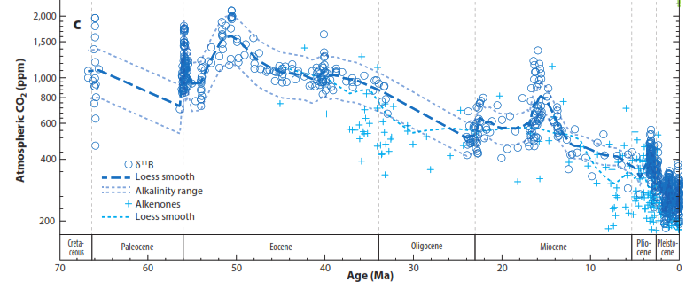
Figure 6. Atmospheric CO2 concentration from proxies for the past 66 million years. Source (Rae, et al., 2021).
CO2 is plant food, more means more plants.
More CO2 fertilizes plants, and they grow faster in the presence of CO2, which is why CO2 is pumped into greenhouses. More CO2 also makes plants more drought resistant. More details here.
Chen, X., Chen, T., He, B., Liu, S., Zhou, S., & Shi, T. (2024). The global greening continues despite increased drought stress since 2000. Global Ecology and Conservation, 49. doi:10.1016/j.gecco.2023.e02791
Zhu, Z., Piao, S., & Myneni, R. (2016). Greening of the Earth and its drivers. Nature Clim Change, 6, 791-795. Retrieved from https://www.nature.com/articles/nclimate3004
CO2 dropped to 180 ppm 20,000 years ago and some plants died of CO2 starvation.
At CO2 partial pressures of 15 Pa or lower (roughly 150 ppm at sea level), most plants will either die or lose their ability to reproduce. In some areas in the last glacial maximum these conditions were possible.
Dippery, J., Tissue, D., & Thomas, R. (1995). Effects of low and elevated CO2 on C3 and C4 annuals. Oecologia, 101, 13-20. Retrieved from https://link.springer.com/article/10.1007/BF00328894
Ice cores can record temperature and CO2.
Alley, R. B. (2000). The Younger Dryas cold interval as viewed from Central Greenland. Quaternary Science Reviews, 19, 213-226. Retrieved from http://klimarealistene.com/web-content/Bibliografi/Alley2000%20The%20Younger%20Dryas%20cold%20interval%20as%20viewed%20from%20central%20Greenland%20QSR.pdf
Neftel, A., Moor, E., & Oeschger, H. (1985). Evidence from polar ice cores for the increase in atmospheric CO2 in the past two centuries. Nature, 315. doi:10.1038/315045a0
Soon, W. (2007). Implications of the Secondary Role of Carbon Dioxide and Methane Forcing in Climate Change: Past, Present, and Future. Physical Geography, 2, 97-125. doi:10.2747/0272-3646.28.2.97
Renee Hannon discusses problems with ice core CO2 estimates here.
CO2 has never driven temperature, it’s the opposite.
See figure 3 and the discussion around it.
Koutsoyiannis, D., Onof, C., Kundzewicz, Z. W., & Christofides, A. (2023). On Hens, Eggs, Temperatures and CO2: Causal Links in Earth’s Atmosphere. Sci, 5(3). doi:10.3390/sci5030035
Soon, W. (2007). Implications of the Secondary Role of Carbon Dioxide and Methane Forcing in Climate Change: Past, Present, and Future. Physical Geography, 2, 97-125. doi:10.2747/0272-3646.28.2.97
The 1930s were very warm.
The most pronounced warming in the historical global climate record, prior to the warming from 1980 to 2000, occurred in the first half of the 20th century. It peaked in the late 1930s.
Hegerl, G. C., Brönnimann, S., Schurer, A., & Cowan, T. (2018). The early 20th century warming: Anomalies, causes, and consequences. WIREs Climate Change, 9(4). doi:10.1002/wcc.522
Climate models do not capture this period of warming very well because they rely too much on CO2. In all likelihood, CO2 played a very small role in the early 20th century warming.
From 1945 to 1976 the world cooled
Guy Callendar published a major paper introducing his collection of past CO2 concentration measurements and global temperatures in 1938. The study tried to show that they correlated in the fashion predicted by Svante Arrhenius thirty years earlier and that CO2 controlled Earth’s temperature. Unfortunately, just after he published the paper the world began to cool as CO2 concentration increased rapidly during the post war industrial boom. The following plot of global temperatures is from HadCRUT4.
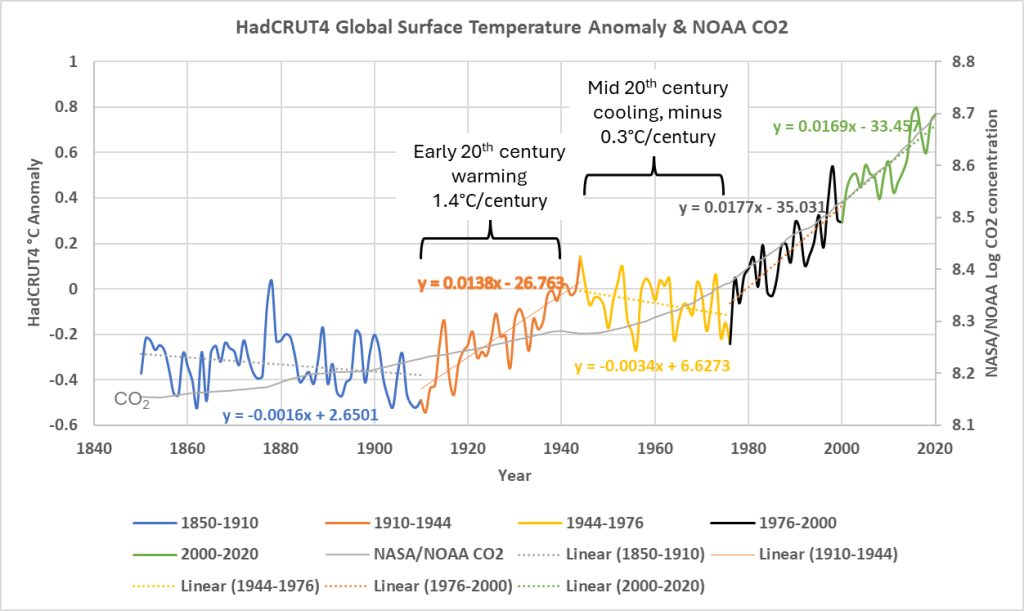
Figure 7. Plot of the HadCRUT4 global surface temperature average and the NOAA/NASA CO2 dataset in light gray. The CO2 concentration is shown as the logarithm to the base two so it can be compared directly to temperature. Notice the correlation is good after 1980, but poor before then.
In figure 7 we see that CO2 increases from about 1945 to 1980 while global average temperature falls.
Arrhenius, S. (1908). Worlds in the Making. (D. H. Borns, Trans.) New York: Harper and Brothers. Retrieved from https://archive.org/details/worldsinmakinge01arrhgoog/page/n7/mode/2up
Callendar, G. S. (1938). The artificial production of carbon dioxide and its influence on temperature. Q. J. R. Meteorol. Soc., 64, 223-240. doi:10.1002/qj.49706427503
HadCRUT4 data here.
Climate models overestimated observed temperature increases.
From the IPCC AR6 WGI report:
“Hence, we assess with medium confidence that CMIP5 and CMIP6 models continue to overestimate observed warming in the upper tropical troposphere over the 1979–2014 period by at least 0.1°C per decade, in part because of an overestimate of the tropical SST trend pattern over this period.“
(AR6 WGI, page 444).
McKitrick, R., & Christy, J. (2018, July 6). A Test of the Tropical 200- to 300-hPa Warming Rate in Climate Models, Earth and Space Science. Earth and Space Science, 5(9), 529-536. doi:10.1029/2018EA000401
McKitrick, R., & Christy, J. (2020). Pervasive Warming Bias in CMIP6 Tropospheric Layers. Earth and Space Science, 7. doi:10.1029/2020EA001281
IPCC. (2021). Climate Change 2021: The Physical Science Basis. In V. Masson-Delmotte, P. Zhai, A. Pirani, S. L. Connors, C. Péan, S. Berger, . . . B. Zhou (Ed.)., WG1. Retrieved from https://www.ipcc.ch/report/ar6/wg1/
Climate models do not reproduce the ocean cycles properly.
From Eade, 2022:
“This suggests that current climate models do not fully represent important aspects of the mechanism for low frequency variability of the NAO.”
Eade, et al. 2022
Eade, R., Stephenson, D., & Scaife, A. (2022). Quantifying the rarity of extreme multi‑decadal trends: how unusual was the late twentieth century trend in the North Atlantic Oscillation? Climate Dynamics, 58, 1555–1568 . doi:10.1007/s00382-021-05978-4
The NAO, the North Atlantic Oscillation, is an important ocean oscillation.
One of the best indicators of the weakness of the CMIP climate models is the fact that they do not reproduce or include as input, these vital climate indicators. For example, see the discussion on the “AMV” (AMV is what AR6 calls the AMO) in AR6 WGI page 504. The “AMV-like” signal in the climate models is too weak, following is a quote from AR6:
“On average, the duration of modelled AMV episodes is too short, the magnitude of AMV is too weak and its basin-wide SST spatial structure is limited by the poor representation of the link between the tropical North Atlantic and the subpolar North Atlantic/Nordic seas. Such mismatches between observed and simulated AMV have been associated with intrinsic model biases in both mean state and variability in the ocean and overlying atmosphere. For instance, compared to available observational data CMIP5 models underestimate the ratio of decadal to interannual variability of the main drivers of AMV, namely the AMOC, NAO and related North Atlantic jet variations … which has strong implications for the simulated temporal statistics of AMV, AMV-induced teleconnections and AMV predictability.”
AR6, page 504
If they can’t model these important oscillations correctly, their models are wrong.
There is no relationship between CO2 concentration and climate.
Besides the lack of a correlation in figure 7, there is also no correlation between CO2 and climate over the entire Holocene as shown in Figure 4 here. This lack of correlation has been called the Holocene Temperature Conundrum.
Kaufman, D., & Broadman, E. (2023, February 15). Revisiting the Holocene global temperature conundrum. Nature, 614, 425-435. Retrieved from https://doi.org/10.1038/s41586-022-05536-w
Liu, Z., Zhu, J., Rosenthal, Y., Zhang, X., Otto-Bliesner, B. L., Timmermann, A., . . . Timm, O. E. (2014). The Holocene temperature conundrum. PNAS, 111. Retrieved from http://www.pnas.org/content/111/34/E3501.short
There is no evidence that the Earth is warmer today than in the past.
See figures 2 and 4 and the references.
There is no evidence that CO2 is now dangerously high.
The CO2 concentration has been many times higher than today in the past, and the only thing that happened was the Earth became greener.
Beerling, D., & Royer, D. (2011). Convergent Cenozoic CO2 history. Nature Geoscience, 4. Retrieved from https://www.nature.com/articles/ngeo1186
Chen, X., Chen, T., He, B., Liu, S., Zhou, S., & Shi, T. (2024). The global greening continues despite increased drought stress since 2000. Global Ecology and Conservation, 49. doi:10.1016/j.gecco.2023.e02791
Zhu, Z., Piao, S., & Myneni, R. (2016). Greening of the Earth and its drivers. Nature Clim Change, 6, 791-795. Retrieved from https://www.nature.com/articles/nclimate3004
Dippery, J., Tissue, D., & Thomas, R. (1995). Effects of low and elevated CO2 on C3 and C4 annuals. Oecologia, 101, 13-20. Retrieved from https://link.springer.com/article/10.1007/BF00328894
Also see this essay on the very warm PETM, 56 million years ago.
Clouds are important in climate change.
Clouds are the largest source of uncertainty in the IPCC calculation of the impact of CO2 concentration on climate according to AR6 WGI page 979. The net impact of changes in average cloud cover ranges from a positive feedback (warming) to a negative or cooling feedback, so even the direction of cloud-caused changes is unknown. Clouds cannot be modeled so their effect must be “parameterized,” which means they are varied in the model according to complex assumptions.
IPCC. (2021). Climate Change 2021: The Physical Science Basis. In V. Masson-Delmotte, P. Zhai, A. Pirani, S. L. Connors, C. Péan, S. Berger, . . . B. Zhou (Ed.)., WG1. Retrieved from https://www.ipcc.ch/report/ar6/wg1/
Koonin, S. E. (2021). Unsettled: What Climate Science Tells us, What it doesn’t, and why it matters. Dallas, Texas, USA: BenBella. Retrieved from https://www.amazon.com/dp/B08JQKQGD5/ref=dp-kindle-redirect?_encoding=UTF8&btkr=1
Ceppi, P., Brient, F., Zelinka, M., & Hartmann, D. (2017, July). Cloud feedback mechanisms and their representation in global climate models. WIRES Climate Change, 8(4). Retrieved from https://onlinelibrary.wiley.com/doi/full/10.1002/wcc.465
Galactic cosmic rays can contribute to creating clouds.
Galactic cosmic rays may help nucleate cloud formation.
Svensmark, H. (1998, November 30). Influence of Cosmic Rays on Earth’s Climate. Physical Review Letters, 81. Retrieved from https://journals.aps.org/prl/abstract/10.1103/PhysRevLett.81.5027
Svensmark, H. (2019). Force Majeure, The Sun’s role in climate change. GWPF. Retrieved from https://www.thegwpf.org/content/uploads/2019/03/SvensmarkSolar2019-1.pdf
Svensmark, H., Svensmark, J., Enghoff, M., & Shaviv, N. (2021). Atmospheric ionization and cloud radiative forcing. Sci Rep, 11. doi:10.1038/s41598-021-99033-1
Nir Shaviv’s spiral arm hypothesis
It is quite possible that Earth’s Ice Ages are related to the solar system’s path through the spiral arms of the Milky Way galaxy as proposed by Nir Shaviv.
Shaviv, N. (2003b). The Spiral structure of the Milky Way, cosmic rays, and ice age epochs on Earth. New Astronomy. Retrieved from http://old.phys.huji.ac.il/~shaviv/articles/long-ice.pdf
Solar wind and its effect on galactic cosmic rays.
Dumbović, M., Vršnak, B., Čalogović, J., & Karlica, M. (2011). Cosmic ray modulation by solar wind disturbances. Astronomy and Astrophysics. doi:10.1051/0004-6361/201016006
Does solar activity correlate with climate changes?
Solar activity correlates with many features of Earth’s climate, including surface temperature, La Nina frequency, and polar vortex strength. For an overview see here.
Connolly et al., R. (2021). How much has the Sun influenced Northern Hemisphere temperature trends? Research in Astronomy and Astrophysics, 21(6). doi:10.1088/1674-4527/21/6/131
Soon, W., Connolly, R., & Connolly, M. (2015). Re-evaluating the role of solar variability on Northern Hemisphere temperature trends since the 19th century. Earth Science Reviews, 150, 409-452. Retrieved from https://www.sciencedirect.com/science/article/pii/S0012825215300349
Soon, W., Connolly, R., Connolly, M., Akasofu, S. I., Baliunas, S., Berglund, J., . . . al., e. (2023). The Detection and Attribution of Northern Hemisphere Land Surface Warming (1850–2018) in Terms of Human and Natural Factors: Challenges of Inadequate Data. Climate, 11(9). doi:10.3390/cli11090179
Connolly et al., R. (2023). Challenges in Detection and Attribution of Northern Hemisphere Surface Temperature Trends since 1850 Research in Astronomy and Astrophysics, 23(10). doi: 10.1088/1674-4527/acf18e
IPCC AR6 cannot attribute extreme weather to humans, but they try.
“… both thermodynamic and dynamic processes are involved in the changes of extremes in response to warming. Anthropogenic forcing (e.g., increases in greenhouse gas concentrations) directly affects thermodynamic variables, including overall increases in high temperatures and atmospheric evaporative demand, and regional changes in atmospheric moisture, which intensify heatwaves, droughts and heavy precipitation events when they occur (high confidence). Dynamic processes are often indirect responses to thermodynamic changes, are strongly affected by internal climate variability, and are also less well understood. As such, there is low confidence in how dynamic changes affect the location and magnitude of extreme events in a warming climate.”
AR6 WGI, page 1527
While AR6 says that it is hard to explain changes in severe weather without anthropogenic forcing, it is “extremely difficult to detect and attribute changes” in precipitation/cyclones/drought/etc. to human activities (AR6 WGI, Chapter 11). They also note that “it remains uncertain whether past changes in Atlantic TC [tropical cyclone] activity are outside the range of natural variability.” AR6 WGI page 1588.
1930s in the U.S. were warmer than today.
This is a complicated issue and no definitive answer can be given either way. The surface temperature data quality and coverage in the U.S. varies a lot since 1930 and the data processing algorithms are often questioned. Further, the differences between the warmest years in the 1930s and today are small and well below the accuracy of the measurements.
James Hansen and a large group of co-authors concluded in 2001 that the U.S. mean temperature had just reached a level comparable to that of the 1930s. He concludes: “The U.S. was warm in 2000 but cooler than the warmest years in the 1930s…”
Hansen, J., Ruedy, R., Sato, M., Imhoff, M., Lawrence, W., Easterling, D., . . . Karl, T. (2001). A closer look at United States and global surface temperature change. Journal of Geophysical Research: Atmospheres, 106(D20), 23947-23963. doi:10.1029/2001JD000354
The U.S. surface temperature data (called USHCN or the U.S. Historical Climatology Network) are ambiguous, and the trend is highly dependent upon the corrections applied to it. Figure 8 compares the final processed CONUS (Contiguous U.S. states) temperature anomaly in blue to the raw temperature anomaly in orange. The important point to notice is that the raw data from the 1930s is nearly as high as raw modern temperatures because the “corrected” data in the 1930s is corrected down and the modern temperatures are “corrected” up. The reasons given for this pattern are controversial. The other unusual thing about the plot is the corrections to the modern data, which is presumably more accurate, are larger than the corrections in the 1930s.
The final temperatures, shown in figure 8 in blue, are highly processed and missing stations are filled in with data from nearby stations. The raw data shown in figure 8 are only the data from real stations, so how many functioning stations exist in any given year matters. Figure 9 shows the number of stations reporting each year in orange. The final station count is forced to be constant by the infilling algorithm.
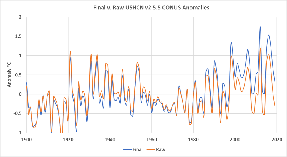
Figure 8. Comparison of the continental U.S. (“CONUS”) USHCN v 2.5.5 weather station
The actual number of reporting weather stations in the 1930s and the 1990s is fairly high and only a few stations had to be infilled with the processing algorithm. Yet while the peak years in the 1930s and in the 1990s have similar raw data temperature anomalies, the final temperatures are different. This is the context behind the statement.
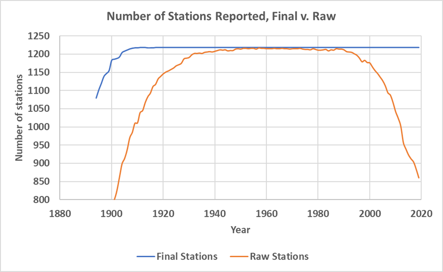
Figure 9. The number of weather stations reporting in each year is shown in orange. Only stations reporting in each of the 12 months of the year are counted to avoid seasonal anomalies. The number of values in the final dataset (some are infilled with the algorithm) are shown in blue. The apparent loss of “accuracy” in figure 8, after 2000 is at least partially due to the loss of reporting weather stations.
More on the U.S. temperature record, including additional references and datasets that indicate the 1930s is warmer than 2000, can be seen here. The post also provides the official explanation for the “corrections.”
James Hansen and co-authors also wrote the following in 1999, link:
“What’s happening to our climate? Was the heat wave and drought in the Eastern United States in 1999 a sign of global warming?
Empirical evidence does not lend much support to the notion that climate is headed precipitately toward more extreme heat and drought. The drought of 1999 covered a smaller area than the 1988 drought, when the Mississippi almost dried up. And 1988 was a temporary inconvenience as compared with repeated droughts during the 1930s “Dust Bowl” that caused an exodus from the prairies, as chronicled in Steinbeck’s Grapes of Wrath.”
(James Hansen, 1999)
Winter temperatures are rising and summer temperatures have hardly changed.
This is a common assumption, but the real story of winter versus summer warming rates is more complex. Models predict that winters and nights will warm faster than summers and days, but this trend only happens in some regions of the Earth. In other areas it is opposite and no one really understands why (Balling, Michaels, & Knappenberger, 1998).
Balling, R., Michaels, P., & Knappenberger, P. (1998). Analysis of winter and summer warming rates in gridded temperature time series. Climate Research, 9. doi:10.3354/cr009175
Wildfires were worse in the 1930s.
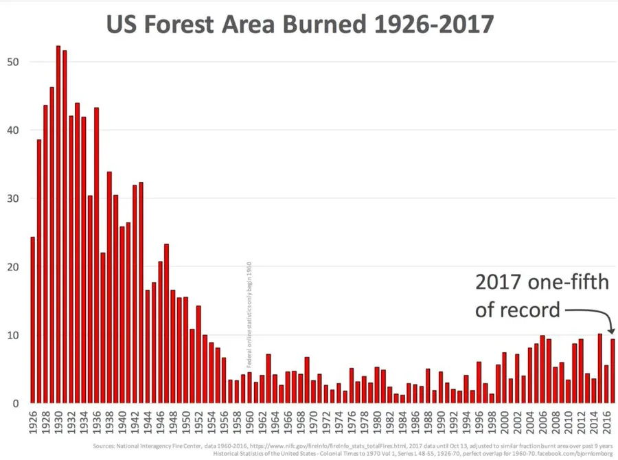
Figure 10. U.S. forest area burned since 1926, from the National Interagency Fire Center.
No change in U.S. hurricanes.
There is no trend or a slight decline in continental U.S. landfalling hurricanes over the past 120 years.
Klotzbach, P. J., Bowen, S. G., Pielke, R., & Bell, M. (2018). Continental U.S. Hurricane Landfall Frequency and Associated Damage: Observations and Future Risks. Bull. Amer. Meteor. Soc, 99, 1359-1376. doi:10.1175/BAMS-D-17-0184.1
No change in global cyclones
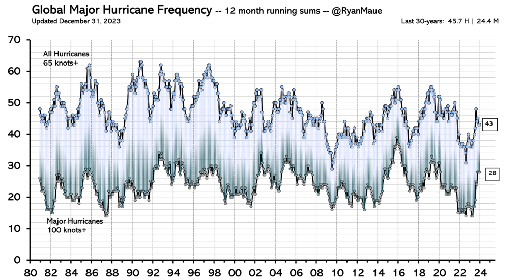
Figure 11. Global major hurricane frequency, from Ryan Maue.
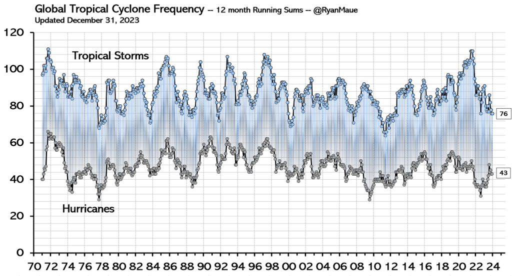
Figure 12. Global tropical cyclone frequency, from Ryan Maue.
Weinkle, J., Maue, R., & Pielke Jr., R. (2012, July 9). Historical Global Tropical Cyclone Landfalls. AMS. doi:https://doi.org/10.1175/JCLI-D-11-00719.1
Antarctic temperatures have not changed.
Schneider, D. P. (2006). Antarctic temperatures over the past two centuries from ice cores. Geophysical Research Letters, 33(16). doi:10.1029/2006GL027057
“Beyond the Antarctic Peninsula there has been little significant change in temperature.”
Turner, et al., 2019
Turner, J., Marshall, G. J., Clem, K., Colwell, S., Phillips, T., & Lu, H. (2019). Antarctic temperature variability and change from station data. International Journal of Climatology, 2986-3007. doi:10.1002/joc.6378
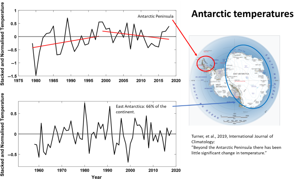
Figure 13. Antarctic temperatures.
Global drought has not changed.
Meteorological drought has not increased in at least the past 120 years.
Vicente-Serrano, S. M., Peña-Angulo, D., Beguería, S., Domínguez-Castro, F., Tomás-Burguera, M., Noguera, I., . . . Ahmed, E. K. (2022). Global drought trends and future projections. Phil. Trans. R. Soc. A, 380. doi:10.1098/rsta.2021.0285
Polar bear population is growing.
As of 2021 the world polar bear population was growing according to polar bear expert Susan Crockford.
Crockford, S. (2022). The State of the Polar Bear 2021. Global Warmig Policy Foundation.
Great barrier reef is growing and reached record levels.
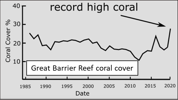
Figure 14. Great Barrier Reef growth record, After Peter Ridd using data from the Australian Institute of Marine Science.
Climate change can kill maple trees?
This is highly speculative, but claimed, see here.
Climate change and prostitution.
Farley, M. (2022). Making the connections: resource extraction, prostitution, poverty, climate change, and human rights. The International Journal of Human Rights, 26(6), 1032-1055. doi:10.1080/13642987.2021.1997999
Climate change affects beer quality.
Mozny, M., Trnka, M., & Vlach, V. (2023). Climate-induced decline in the quality and quantity of European hops calls for immediate adaptation measures. Nature. doi:10.1038/s41467-023-41474-5
Climate change in video games.
Yes, there are climate change video games, see here and here.
If you don’t find climate change is a problem your money dries up.
Koonin, S. E. (2021). Unsettled: What Climate Science Tells us, What it doesn’t, and why it matters. Dallas, Texas, USA: BenBella. Retrieved from https://www.amazon.com/dp/B08JQKQGD5/ref=dp-kindle-redirect?_encoding=UTF8&btkr=1
On page 202 of Koonin’s book we find this:
“On March 7, 2019, Senator Schumer (together with Senators Carper, Reed, Van Hollen, White-house, Markey, Schatz, Smith, Blumenthal, Shaheen, Booker, Stabenow, Klobuchar, Hassan, Merkley, and Feinstein) introduced Senate bill S.729:”
“ . . . to prohibit the use of funds to Federal agencies to establish a panel, task force, advisory committee, or other effort to challenge the scientific consensus on climate change, and for other purposes.”
Koonin, 2021, p 202
Incredibly shocking, the U.S. Senate attempting to legislate scientific research outcomes, it doesn’t get worse than this. Fortunately, the bill failed to pass, but the political pressure to find human’s caused recent climate changes is overwhelming.
Filing reports on how climate change affects businesses.
The U.S. SEC have tried to implement a new climate change impact filing requirement, see here. However the rule has been temporarily halted by the courts (see here).
It has been criticized as unnecessarily punitive and expensive.
Renewable energy is a trillion-dollar business.
A recent McKinsey report expects $9.2 trillion to be spent on reaching net zero by 2050.
Download the report here.
70,000 people went to IPCC meeting Dubai 2023
70,000 global leaders, climate activists, and billionaires go to Dubai meeting.
Explosion of climate change jobs
New government climate change jobs.
Linkedin data shows hiring for green jobs consistently outpaces overall hiring according to the World Economic Forum.
How much does the sun change.
Scafetta, N. (2023c, July 6). Understanding the role of the sun in climate change. Retrieved from andymaypetrophysicist.com: https://andymaypetrophysicist.com/2023/07/06/understanding-the-role-of-the-sun-in-climate-change/
Scafetta, N., & Willson, R. (2014). ACRIM total solar irradiance satellite composite validation versus TSI proxy models. Astrophysics and Space Science, 350(2), 421-442. Retrieved from https://link.springer.com/article/10.1007/s10509-013-1775-9
Soon, W., Connolly, R., & Connolly, M. (2015). Re-evaluating the role of solar variability on Northern Hemisphere temperature trends since the 19th century. Earth Science Reviews, 150, 409-452. Retrieved from https://www.sciencedirect.com/science/article/pii/S0012825215300349
Connolly et al., R. (2023). Challenges in Detection and Attribution of Northern Hemisphere Surface Temperature Trends since 1850 Research in Astronomy and Astrophysics, 23(10). doi: 10.1088/1674-4527/acf18e
We are looking for the range of natural variability.
“… a significant part of the 20th century warming may be interpreted as the result of natural climatic variations…”
Humlum, 2011
Humlum, O., Solheim, J.-E., & Stordahl, K. (2011). Identifying natural contributions to late Holocene climate change. Global and Planetary Change, 79(1), 145-156. doi:10.1016/j.gloplacha.2011.09.005
Here is a discussion of natural variability in the Arctic by Judith Curry.
“These results support the notion that the enhanced wintertime warming over high northern latitudes from 1965 to 2000 was mainly a reflection of unforced variability of the coupled climate system.”
(Wallace, Qiang, Smoliak, & Johanson, 2012)
Wallace, J., Q. F., Smoliak, B. V., & Johanson, C. M. (2012). Simulated versus observed patterns of warming over the extratropical Northern Hemisphere continents during the cold season. Earth, Atmospheric, And Planetary Sciences, 109(36). doi:10.1073/pnas.1204875109
More government control.
“The politician’s power increases because exercising power increases it and people will give up their freedoms in exchange for security, whether the danger is real or not.”
(May, Politics and Climate Change: A History, 2020c, p. 15)
May, A. (2020c). Politics and Climate Change: A History. Springfield, Missouri: American Freedom Publications.
“No matter if the science of global warming is all phony…climate change [provides] the greatest opportunity to bring about justice and equality in the world.”
Christine Stewart, Canadian Minister of the Environment, speaking to the editors and reporters of the Calgary Herald in 1998.
“This is the first time in the history of mankind that we are setting ourselves the task of intentionally, within a defined period of time to change the economic development model that has been reigning for at least 150 years, since the Industrial Revolution.”
Christiana Figueres, February 4th, 2015
None of the countries participating in the 1997 Kyoto Protocol had any idea what the treaty would cost them, either in jobs or standard of living. They also had no idea what the benefits would be. William Nordhaus, the famous Yale economist and Nobel laureate, called the Kyoto Protocol a:
“conceptual disaster; it has no coherence politically or economically or environmentally.”
William Nordhaus, (Yale University, 2007, pp. 131-132).
Kyoto had little to do with climate change, it was mainly an enormous transfer of money from wealthy countries to poor countries. (May, Politics and Climate Change: A History, 2020c, pp. 236-237)
Yale University. (2007). Yale Symposium on the Stern Review. Retrieved from http://piketty.pse.ens.fr/files/SternReviewYaleSymposium2007.pdf
What stove can you have.
Bans on natural gas stoves, furnaces, and hot water heaters.
What car can you drive.
The push to force people to buy EVs
Burning wood and dung for heat or to cook is deadly.
“Traditional biofuels” are the burning of wood and dung in houses or businesses for heat, light, or cooking. This is not desirable because it produces toxic air pollution. The indoor air pollution caused by traditional biofuels, causes 4% of global deaths. A major study, published in The Lancet, estimates that more than two million deaths can be attributed to indoor air pollution in 2019 (Christopher Murray, 2020). The World Health Organization (WHO) estimates that four million deaths, every year, are caused by indoor air pollution. Domestic wood burning is not just a problem in the developing world, the European Environment Agency, WHO, and the Netherlands Organization for Applied Scientific Research suggest that over 40% of toxic emissions are from residential biomass burning. The UK Department for Environment, Food, and Rural affairs (DEFRA) estimates that 38% of UK air pollution is due to wood-burning stove emissions.”
More discussion here.
Fossil fuels drive agriculture
“The energy-intensiveness of industrial agriculture is well-documented”
“The energy basis of industrial food production has a rich tradition, but quantitative analysis of changes in energy use in agriculture has been limited by the lack of consistent data. This analysis used a new methodology for calculating the direct and indirect use of fossil fuels in agriculture. The procedure was used to quantify energy use in USA agriculture from 1910 to 1990. The results showed a substantial overall increase in energy use from 1910 through the 1970s, and a shift from gasoline to diesel fuel and electricity. The use of all fuels declined in the 1980s.”
“Energy productivity rose in the 1980s due to a diminution in the rate of energy use, a reduction in the number of harvested acres, and larger farms. The results showed a clear response of farmers to higher energy prices that resulted in technical and managerial changes that improved energy productivity.”
(Cleveland, 1995)
In essence the higher energy prices in the 1980s led to small farmers selling out to larger more efficient farmers, improving overall productivity. Small farmers being forced to sell out to larger farmers was epidemic in the 1980s and mostly due to the high cost of gasoline and diesel.
Cleveland, C. (1995, September). The direct and indirect use of fossil fuels and electricity in USA agriculture, 1910-1990. Agriculture, Ecosystems and Environment, 111-121. doi:10.1016/0167-8809(95)00615-Y
Fossil fuels built western civilization.
The 20th century has been called the “Age of Oil” and with good reason. It was a century when life expectancy doubled and extreme poverty dropped from 80% to less than 10%. The drop in poverty is closely correlated (R2= 0.99) to fossil fuels consumed.
Yergin, D. (1991). The Prize. New York: Touchstone.
Yergin, D. (2011). The Quest. New York: Penguin.
Green agenda is ruthless.
The inhumanity of the green agenda.
“In recent years, the overused word ‘sustainability’ has fostered a narrative in which human needs and aspirations have taken a back seat to the green austerity of Net Zero and ‘degrowth’. The ruling classes of a fading West are determined to save the planet by immiserating their fellow citizens. Their agenda is expected to cost the world $6 trillion per year for the next 30 years. Meanwhile, they will get to harvest massive green subsidies and live like Renaissance potentates.”
See Joel Kotkin, Spiked, here for more.
China builds two coal powerplants a week.
In 2022 China granted permits for 106 coal power plants across 82 sites.
China uses more coal than the rest of the world combined.
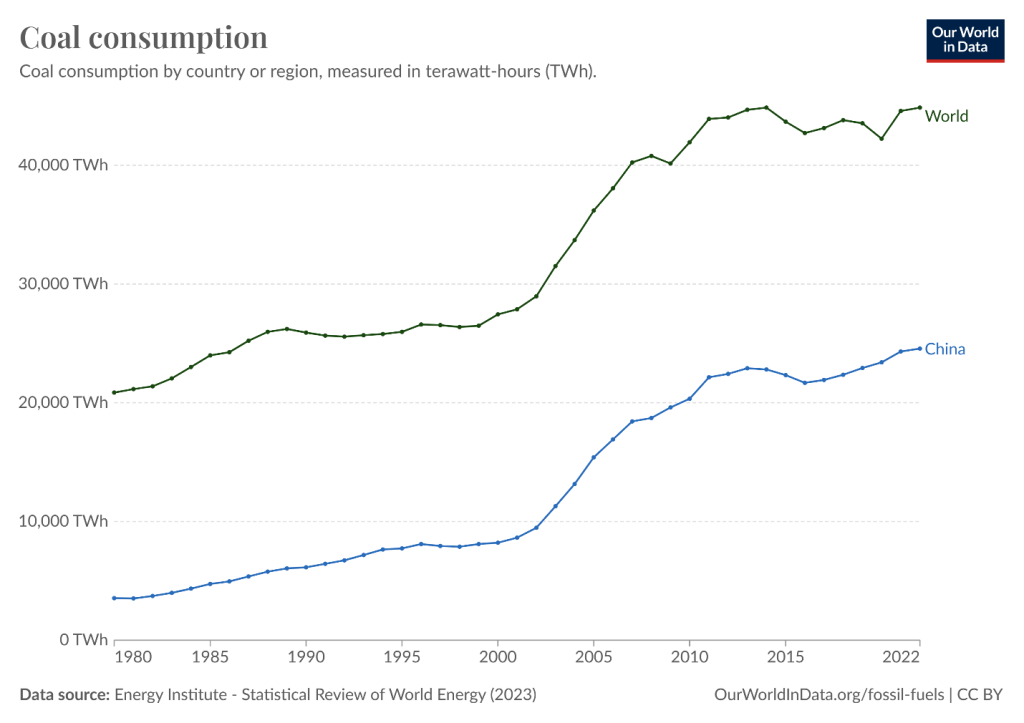
Figure 15. Coal consumption for the whole world compared to China from ourworldindata.org.
Anti-environmentalism is rampant.
Polish farmers protest EU environmental regulations.
Belgian farmers protest excessive environmental rules.
The European protests are affecting policy.
A full bibliography, in traditional alphabetical order can be downloaded here.
