Sea surface and mixed layer temperatures

As described in my previous post, the ocean “mixed layer” is sandwiched between the very thin “skin” layer at the ocean surface and the deep ocean. The skin layer loses thermal energy (“heat”) to the atmosphere primarily through evaporation, gains thermal energy from the Sun during the day, and constantly attempts to come to thermal equilibrium with the atmosphere above it. During the day, with the Sun beating down on the ocean and calm clear conditions, the skin layer might be as thick as ten meters. At night, especially under windy conditions, it can be less than a millimeter thick.

The mixed layer is a zone where turbulence, caused by surface currents and wind has so thoroughly mixed the water that temperature, density, and salinity are relatively constant throughout the layer. Originally, the “mixed layer depth,” the name for the base of the layer, was defined as the point where the temperature was 0.5°C different from the surface (Levitus, 1982). This was found to be an inadequate definition near the poles in the winter, because the temperature there, in certain areas, can be nearly constant to 2,000 meters, but the mixed layer turbulent zone isn’t that deep (Holte & Talley, 2008). Two of the areas that create problems when picking the mixed layer depth with the 0.5°C criteria are the North Atlantic, between Iceland and Scotland and in the Southern Ocean southwest of Chile. The areas are noted with light blue boxes in Figure 1.

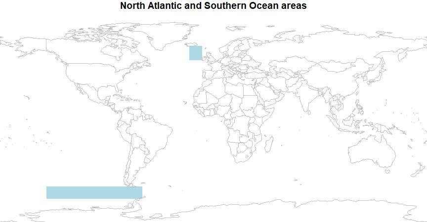
Figure 1. The North Atlantic and Southern Ocean areas where defining the mixed layer depth is difficult because of downwelling surface water during the local winter.

The regions shown in Figure 1 are areas where significant downwelling of surface water to the deep ocean takes place, these are not the only areas where this happens, but these areas often contain nearly constant temperature profiles for the upper 1,000 meters, or even deeper. Figure 2 shows the average July temperature profile for the Southern Ocean area in Figure 1.

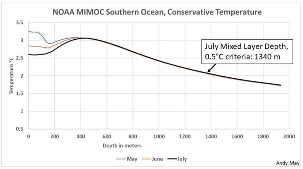
Figure 2. A Southern Ocean July average temperature profile from the blue region shown in Figure 1. The data used to make the profile is from more than 12 years, centered on 2008. Data from NOAA MIMOC.

As explained by James Holte and Lynne Talley (Holte & Talley, 2008), the deep convection in this part of the Southern Ocean has distorted the temperature profile to such an extent that a simple temperature cutoff cannot be used to set the mixed layer depth. Numerous solutions to the problem have been proposed over the years and these are listed and discussed in their article. Their proposed methodology is used by Sunke Schmidtko to define the mixed layer in the NOAA MIMOC dataset discussed below (Schmidtko, Johnson, & Lyman). The Holte and Talley method is complicated, as are many of the other solutions. It does not seem that a generally accepted methodology for defining the mixed layer has been found to date.

Depending upon location and season, the mixed layer depth changes. It is thickest in the local winter in the higher latitudes. There it can extend to 400 meters below the surface or farther using the Holte and Talley logic, and much deeper using the 0.5°C temperature cutoff. Figure 3 shows a map of the mixed layer depth in January.

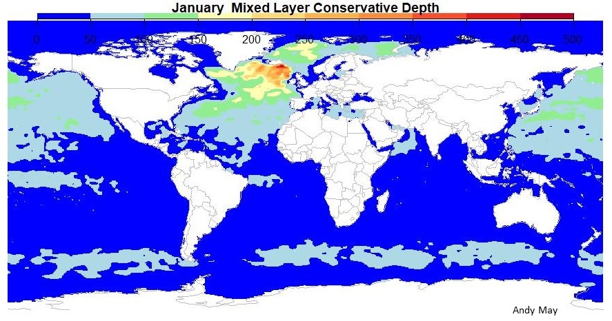
Figure 3. Ocean mixed layer depth in January using the Holte and Talley logic. The oranges and reds are 400 to 500 meters. Data from NOAA MIMOC.

However, the Northern Hemisphere mixed layer thickness thins during the northern summer months and it thickens in the Southern Hemisphere, especially in the Southern Ocean surrounding Antarctica, as shown in Figure 4.

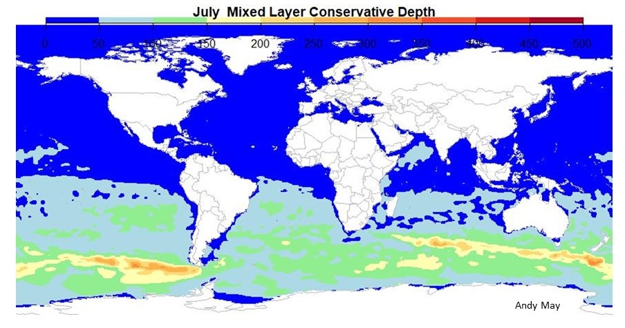
Figure 4. The ocean mixed layer depth in July using the Holte and Talley logic. Again, the oranges and reds are 400 to 500 meters. Data from NOAA MIMOC.

The thicker mixed layer zones always occur in the local winter and reach their peak near 60° latitude as seen in Figure 5.

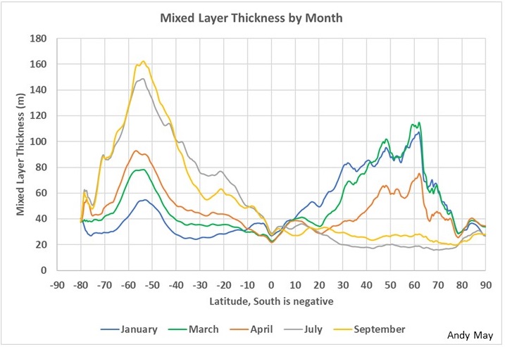
Figure 5. Average mixed layer thickness by latitude and month. The thickest mixed layer is reached in the Southern Hemisphere at about 55 degrees south. In the Northern Hemisphere the peak is reached around 60 degrees. The mixed layer depth in this plot is computed using the methodology developed by Holte and Talley. Data from NOAA MIMOC.

The significance of the Mixed Layer
In our previous post, we emphasized that the mixed layer is in thermal contact with the atmosphere, with a small delay of a few weeks. It also has about 22 times the heat capacity of the atmosphere, which smooths out the radical changes in atmospheric temperature caused by weather events. Thus, when looking at climate, which is much longer term than weather, observing the trend in mixed layer temperature seems ideal. In Figure 6 we compare the yearly global average mixed layer temperature from Jamstec, MIMOC and the University of Hamburg to the global sea-surface temperature (SST) estimates from the Hadley Climatic Research Unit and NOAA. These are not anomalies, these are actual measurements, but they are all corrected and gridded. I have simply averaged the respective global grids.

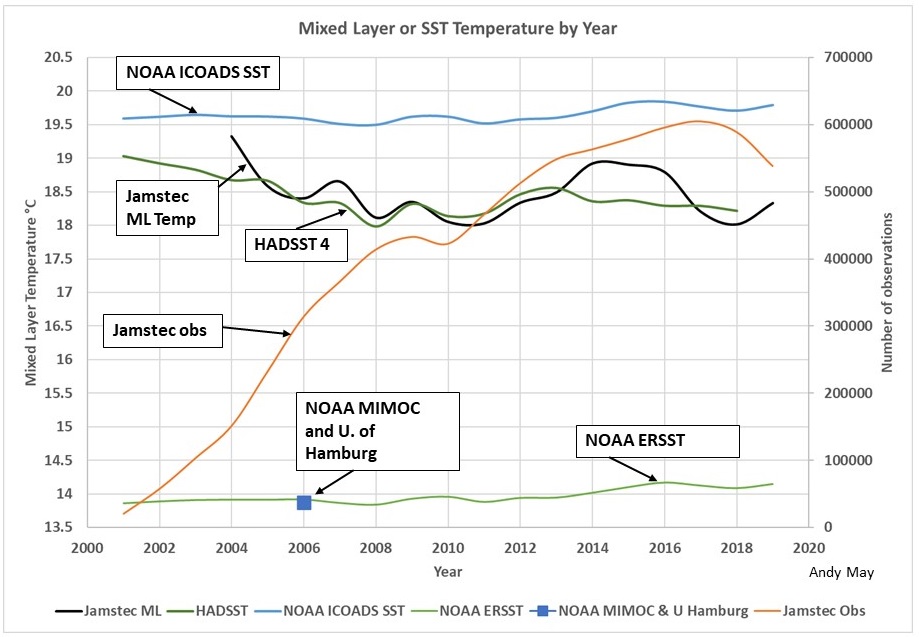
Figure 6. The Jamstec computed global mixed layer temperature is plotted in black. It is compared to HadSST version 4, NOAA’s ICOADS SST, and NOAA’s ERSST. NOAA MIMOC, and the University of Hamburg’s mixed layer temperatures are nearly identical and centered on 2006, they are plotted as a boxes, which overly one another. Data is from the respective agencies.

Decent ocean coverage is only available since 2004, so the years before then are suspect. In Figure 6, all data are plotted as yearly averages. The Hadley CRU temperatures agree well with the Jamstec mixed layer record and, surprisingly, both records show similar declining temperature trends of about two to three degrees per century. NOAA’s ICOADS (International Comprehensive Ocean-Atmosphere Data Set) SST trend is flat to increasing and over a degree warmer than the other two records. The number of Jamstec mixed layer observations are plotted in orange (right scale) to help us judge the data quality for each year. Jamstec reached 150,000 observations in 2004 and we held the subjective opinion that this was enough.

The NOAA MIMOC and University of Hamburg mixed layer temperatures are much lower than HadSST and the Jamstec mixed layer temperatures. Yet, these two multi-year averages, that are centered on 2006, fall right on top of the ERSST SST record and they are over four degrees lower than HaddSST and Jamstec. The difference cannot be simply where the temperatures are taken. It can’t even be in the data, all these records use nearly the same input raw data, it must be in the corrections and methods.

The various mixed layer temperature estimates are different and so are the SSTs. Why are two records declining and the rest flat or increasing? The different estimates do not agree on temperature or trend.

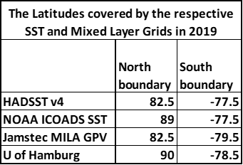
Sea surface and mixed layer temperatures should not need to be turned into anomalies unless they are compared to terrestrial temperatures. They are all taken at approximately the same elevation and in the same medium. All the datasets are global, with similar input data. All are gridded to reduce the impact of uneven data distribution. The grids are different sizes and the gridded areas do differ in their northern and southern limits, but all the grids cover all longitudes. Table one lists the latitude data limits of the grids, they aren’t that different.

Table 1. The north and south data limits for each dataset in 2019.

 

In Figure 7 we have plotted the HadSST and ERSST anomalies. How did they get these anomalies from the measurements in Figure 6?

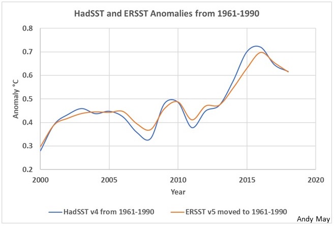
Figure 7. HadSST and ERSST version 4 temperature anomalies.

The HadSST record is maintained by John Kennedy and his colleagues at the MET Hadley Climatic Research Unit (Kennedy, Rayner, Atkinson, & Killick, 2019). They note that their record is different from ERSST and admit it is due to the difference in corrections and adjustments to the raw data. Kennedy mentions that SST “critically contributes to the characterization of Earth’s climate.” We agree. Kennedy also writes that:

“One of the largest sources of uncertainty in estimates of global temperature change is that associated with the correction of systematic errors in sea-surface temperature (SST) measurements. Despite recent work to quantify and reduce these errors throughout the historical record, differences between analyses remain larger than can be explained by the estimated uncertainties.” (Kennedy, Rayner, Atkinson, & Killick, 2019)

One glance at Figure 6 verifies this statement is correct. Most of Kennedy’s 90-page paper catalogues the difficulties of building an accurate SST record. He notes that even subtle changes in the way SST measurements are made can lead to systemic errors of up to one degree, and this is the estimated 20^th century global warming. We do not believe the SST record from 1850 to 2005 is worthwhile. The ambiguous data sources (mainly ships and buckets to WWII and ship intake temperatures after) and the imprecise corrections swamp any potential climate signal. The data is much better since 2005, but Figure 6 shows wide differences in compilations from different agencies. Next, we review the agency definitions of the variables plotted in Figure 6.

Met Office Hadley Centre HadSST 4 data set.
This data was read from a HadSST NetCDF file. NetCDF files are the way most climate data are delivered, I’ve explained how to read them with R (a high quality free statistical program) in a previous post. The variable read from the HadSST file was labeled “tos,” it is a 5-degree latitude and longitude grid defined as “sea water temperature.” The documentation says it is the ensemble-median sea-surface temperature from HadSST v4. The reference given is the paper by John Kennedy already mentioned (Kennedy, Rayner, Atkinson, & Killick, 2019). HadSST uses data from ICOADS release 3, supplemented by drifting buoy data from the Copernicus Marine Environment Monitoring Service (CMEMS). Kennedy mentions the difference between his dataset and ERSST v5 seen clearly in Figure 6. The Hadley Centre SST is corrected to a depth of 20 cm.

NOAA ERSST v5
In Figure 6 we plot yearly global averages of the ERSST v5 NetCDF variable “sst,” which is defined as the “Extended reconstructed sea surface temperature.” They note that the actual measurement depth varies from 0.2 to 10 m, but all measurements are corrected to the optimum buoy measurement depth of 20 cm, precisely the same reference depth as HadSST. Also, like HadSST, ERSST takes its data from ICOADS release 3 and utilizes Argo float and drifting buoys between 0 and 5 meters to compute SST. This makes sense, since ERSST agrees with the University of Hamburg dataset and NOAA’s MIMOC (mixed layer) datasets, which also rely heavily on Argo float data. As discussed above, SST (at 20 cm) and the mixed layer temperature should agree closely with one another almost all the time. The ERSST anomalies plotted in Figure 7 are from the variable “ssta.” I moved ssta to the HadSST reference period of 1961-1990, from the original reference of 1970-2000. The basic reference to ERSST v5 is a paper by Boyin Huang and colleagues (Huang, et al., 2017).

Like Kennedy, Boyin Huang directly addresses the differences between ERSST and HadSST. Huang believes that the differences are due to the different corrections to the raw data applied by the Hadley Centre and NOAA.

NOAA MIMOC
The global average NOAA MIMOC mixed layer “conservative temperature” is plotted in Figure 6 as a box that falls on the ERSST line. It is plotted as one point in 2006 because the MIMOC dataset uses Argo and buoy data over more than 12 years centered on that year. The global average temperature of all that data is 13.87°C from 0 to 5 meters depth. Conservative temperature is not the same as SST. SST is measured, conservative temperature is computed such that it is consistent with the heat content of the water in the mixed layer and takes into account the water salinity and density. However, we would expect SST to be very close to the conservative temperature. Since the conservative temperature more accurately characterizes the heat content of the mixed layer, it is more useful than SST for climate studies. The primary reference for this dataset is the already mentioned paper by Schmidtko (Schmidtko, Johnson, & Lyman).

University of Hamburg dataset
The University of Hamburg dataset is similar to MIMOC in that it is not divided by year, but pools all available data over the past 20 to 40 years to make a high resolution dataset and set of grids of ocean temperature by depth. Like ERSST and MIMOC it relies heavily on Argo and buoy data. The global average temperature of the upper five meters of the oceans in this data set is 13.88°C, barely different from the MIMOC value. The NetCDF variable used is “temperature.” It is defined as the “optimally interpolated temperature.” The documentation states that the zero depth is SST, it is not “conservative temperature.” However, the value is nearly identical to conservative temperature. The main reference for this data set is an Ocean Science article by Viktor Gouretski (Gouretski, 2018).

NOAA ICOADS
The NOAA ICOADS line in Figure 6 is downloaded from the KNMI Climate Explorer and labeled “sst.” The description is: “Sea Surface Temperature Monthly Mean at Surface.” ICOADS version 3 data is used in all the other agency datasets described here, but the organization does not do a lot of analysis. By their own admission they provide a few “simple gridded monthly summary products.” Their line is shown in Figure 6 for reference, but it is not a serious analysis and probably should be ignored. It does help show how imprecise the data is.

Jamstec ML Temperature
The Jamstec MILA GPV product lines up well with HadSST as can be seen in Figure 6. This line is from the NetCDF variable “MLD_TEMP.” It is the central temperature of the mixed layer. The temperature is not a true “conservative temperature,” but the way it is computed ensures that it will be close to that value. The reference for this product is a Journal of Oceanography article by Shigeki Hosada and colleagues (Hosada, Ohira, Sato, & Suga, 2010). Jamstec uses mostly Argo float and buoy data.

Conclusions
The total temperature spread shown in Figure 6 is over 5.5°C and yet these agencies are starting with essentially the same data. This is not an attempt to characterize the SST and mixed layer temperature one-hundred years ago, these are attempts to tell us the average ocean surface temperature today. To put Figure 6 into perspective, the total heat content of our atmosphere is roughly 1.0×10²⁴ Joules, the difference between the HadSST line in Figure 6 and the ERSST line, assuming an average mixed layer depth of 60 meters (from Jamstec), is 3.9×10²³ Joules or nearly 39% of the total thermal energy in the atmosphere.

I have no idea whether HadSST’s or ERSST’s temperatures are correct. They cannot both be correct. I lean toward the ERSST temperatures since it is hard to have an 18-degree ocean in a 15-degree world, but then why are the HadSST temperatures so high? The single most important variable in determining how quickly the world is warming or cooling is the ocean temperature record. We have better data available since about 2004, but obviously no agreed method of analyzing it. When it comes to global warming (or, perhaps, global cooling) the best answer is we don’t know.

Given that oceans cover 71% of the Earth’s surface and contain 99% of the heat capacity, the differences in Figure 6 are enormous. These discrepancies must be resolved, if we are ever to detect climate change, human or natural.

I processed an enormous amount of data to make this post, I think I did it correctly, but I do make mistakes. For those that want to check my work, you can find my R code here.

None of this is in my new book Politics and Climate Change: A History but buy it anyway.

You can download the bibliography here.